In this post, I am going to share with you my understanding in Restricted Boltzmann Machine (RBM).
Restricted Boltzmann Machine is a stochastic artificial neural network that learns the probability distribution of input. A stochastic artificial neural network means a structure contains a series of units with values between 0 to 1 that depend on weights and adjacent units [8]. From a high level, RBM encodes the information of input into weights and hidden values.
Let’s see one example given in [8]:
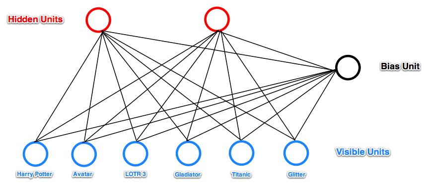
In this example, RBM tries to learn hidden factors of a user given his movie watch list. When input a watch list, the RBM has the hidden units activated or not depending on whether the input passing through the weights can reach a value high enough to activate the sigmoid function. On the other hand, after you infer hidden unit values from the input, you can infer which input units, not observed in the input yet, is most likely to activate.
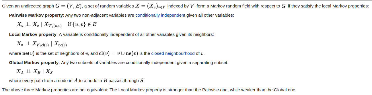
RBM is also a special case of undirected graphical model which we call Markov Random Field (MRF). An undirected graphical model must satisfy three Markov properties to be called MRF:
If we call all variables of an MRF $latex x \in \mathcal{R}^k$, then the joint distribution of the MRF can be formulated as [9]:
$latex P(x)= \frac{1}{Z}\prod\limits_{c \in C} \phi_c(x_c)= \frac{1}{Z}\prod\limits_{c \in C} e^{-E(x_c, \theta_c)} &s=2$
, where $latex C$ is a set of cliques of the MRF, $latex E(x_c, \theta_c)$ is an energy function parameterized by $latex \theta_c$, $latex Z$ is a normalization term, i.e. $latex Z=\sum\limits_x \prod\limits_{c \in C} e^{-E(x_c, \theta_c)}$.
A few more words on energy function: an energy function $latex E(x, \theta)$ returns a scalar representing the “energy” of $latex x$ under the parameterization of $latex \theta$. You can think $latex E(x, \theta)$ as an unnormalized measurement of how unlikely a data point $latex x$ is generated by the distribution controlled by $latex \theta$. The smaller $latex E(x, \theta)$ it is, the more possible $latex x$ is generated by $latex \theta$. Analogous to physics, the higher energy an object has, the more unstable the object is. An tutorial of energy function can be found in [2].
If we name all input units as a vector $latex v \in \mathcal{R}^{m}$ and all hidden units as a vector $latex h \in \mathcal{R}^{n}$, then the energy function of the RBM is:
$latex E(v, h, \Theta) = -b^T v – c^T h – h^T W v &s=2$
, where $latex b$ is the vectorized bias of $latex v, $latex c$ is the vectorized bias of $latex h$, $latex W$ are weight matrix in which $latex w_{ij}$ connects visible unit $latex V_j$ and hidden unit $latex H_i$ and $latex \Theta = \{W, c, b\}$. By the definition of energy function, you can say the most probable $latex v$ and $latex h$ are the variables that jointly minimize $latex E(v, h, \Theta)$, which is the linear combination of $latex v$, $latex h$ and the RBM’s parameters $latex W$, $latex c$ and $latex b$. If $latex W$, $latex c$ and $latex b$ can be learned really well to capture the relationship between $latex v$ and $latex h$, then we can infer $latex h$ given $latex v$, or vice versa, reconstruct $latex v$ given $latex h$.
Why is $latex E(v, h, \Theta)$ defined in this way, namely, a linear combination of $latex v$, $latex h$, $latex W$, $latex c$ and $latex b$? I am not fully understood about it but there are ongoing discussion online: [10] [11]. What I guess is that the designer considers: (1) the simplicity of linearity; (2) the idea from Hopfield Network given in [12]. You should know clearly that in an RBM each pair of adjacent hidden unit and input unit forms a clique. $latex E(v, h, \Theta)$ defined above is actually the sum of the energy function of each pair of hidden unit and input unit. That is, $latex E(v, h, \Theta)$ can be rewritten as:
$latex E(v, h, \Theta) = -\sum\limits^n_{i=1}\sum\limits_{j=1}^m w_{ij}H_i v_j – \sum\limits_{j=1}^m b_j v_j – \sum\limits_{i=1}^n c_i h_i &s=2$
The difficulty in RBM is the learning process. Let’s look at its objective function, log-likelihood of $latex \Theta$ and observed data. To simplify, we write the log-likelihood when there is only one data point, $latex v \in R^m$:
$latex ln \mathcal{L}(\Theta, v)=ln\frac{1}{Z}\sum\limits_h e^{-E(v, h)} = ln \sum\limits_h e^{-E(v,h)} – ln\sum\limits_{\tilde{v},h}e^{-E(\tilde{v},h)}&s=2$
Its derivative regarding $latex \Theta$ is:
$latex \frac{\partial ln \mathcal{L}(\Theta, v)}{\partial \Theta}= \frac{\partial}{\partial \Theta}(ln \sum\limits_h e^{-E(v,h)}) – \frac{\partial}{\partial \Theta}(ln\sum\limits_{\tilde{v},h}e^{-E(\tilde{v},h)})\\ =-\frac{1}{\sum\limits_h e^{-E(v,h)}}\sum\limits_h e^{-E(v,h)} \frac{\partial E(v,h)}{\partial \Theta} + \frac{1}{\sum\limits_{\tilde{v},h}e^{-E(\tilde{v},h)}}\sum\limits_{\tilde{v},h}e^{-E(\tilde{v},h)} \frac{\partial E(\tilde{v},h)}{\partial \Theta} \\=-\sum\limits_h p(h|v) \frac{\partial E(v,h)}{\partial \Theta} + \sum\limits_{\tilde{v},h} p(\tilde{v},h) \frac{\partial E(\tilde{v},h)}{\partial \Theta} &s=2$
Note that the first term involves the summation of all possible states of hidden units given a specific $latex v$ vector. The second term involves the summation of all states of both hidden units and visible units. This makes the derivation expensive to calculate!
Using some factorization trick (equation 28 in [6], note equation 28 should have one more negative sign), one can obtain the alternative formulas to calculate derivatives (equation 29, 32 & 33 in [6]):
$latex \frac{\partial ln \mathcal{L}(\Theta,v)}{\partial w_{i,j}} =-\sum\limits_h p(h|v) h_i v_j + \sum\limits_{\tilde{v},h} p(\tilde{v}, h) h_i\tilde{v}_j \\ = p(H_i=1|v)v_j – \mathbb{E}_{p(\tilde{v})} [p(H_i=1|\tilde{v})\tilde{v}_j] &s=2$
$latex \frac{\partial ln \mathcal{L}(\Theta,v)}{\partial b_j} = v_j – \sum\limits_{\tilde{v}} p(\tilde{v})\tilde{v}_j \\ \qquad \qquad = v_j – \mathbb{E}_{p(\tilde{v})}\tilde{v}_j &s=2$
$latex \frac{\partial ln \mathcal{L}(\Theta, v)}{\partial c_i} = \sum\limits_h p(h|v) h_i – \sum\limits_{\tilde{v}} p(\tilde{v}) \sum\limits_h p(h|\tilde{v}) h_i \\=p(H_i=1|v)-\mathbb{E}_{p(\tilde{v})} p(H_i=1|\tilde{v}) &s=2$
However, the computation complexity can only be reduced to exponential size of visible units (instead of combination of visible and hidden states). However this is still intractable. If we use “Contrastive Divergence” (CD), we can approximate those expectations. In a k-step CD, each step t consists of sampling $latex h^{(t)}$ from $latex p(h|v^{(t)})$ and sampling $latex v^{(t+1)}$ from $latex p(v|h^{(t)})$. $latex v^{(0)}$ is set as the original training sample. The procedure is as follows:
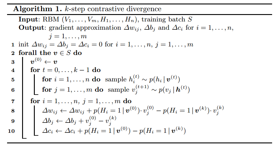
After obtaining the output of k-step CD, the gradient approximation $latex \nabla w_{ij}$, $latex \nabla b_j$ and $latex \nabla c_i$, we can update $latex \Theta$ by gradient ascent because we want to maximize $latex \mathcal{L}(\Theta, v)$.
Now let’s look at [1], a piece of Theano code implementing RBM. It actually shows similar introduction why approximation methods such as contrastive divergence are needed when training RBM.
First, let’s get familiar with some notations. [1] introduces free energy of visible units:
$latex \mathcal{F}(v) = -log \sum\limits_h e^{-E(v,h,\Theta)}$
Then, when given an arbitrary input $latex v \in \mathbb{R}^m$, the negative log likelihood can be written in the form of $latex \mathcal{F}(v)$ (equation 4 in [1]):
$latex – \frac{\partial log \mathcal{L}(\Theta, v)}{\partial \Theta} \\= -\partial \log \frac{e^{-\mathcal{F}(v)}}{\sum\limits_{\tilde{v}}e^{-\mathcal{F}(v)}} / \partial \Theta \\= \frac{\partial \mathcal{F}(v)}{\partial \Theta} – \sum\limits_{\tilde{v}} \frac{ e^{-\mathcal{F}(\tilde{v})}}{\sum\limits_{\tilde{v}} e^{-\mathcal{F}(\tilde{v})}} \frac{\partial \mathcal{F}(\tilde{v})}{\partial \Theta} \\=\frac{\partial \mathcal{F}(v)}{\partial \Theta} – \sum\limits_{\tilde{v}}p(\tilde{v})\frac{\mathcal{F}(\tilde{v})}{\partial \Theta}\\= \frac{\partial \mathcal{F}(v)}{\partial \Theta} – E_P[\frac{\partial \mathcal{F}(\tilde{v})}{\partial \Theta}]&s=2$
Since it is given in negative log likelihood, we want it as small as possible. Here is the intuition explained in [1]: The first term increases the probability of training data (by reducing the corresponding free energy), while the second term decreases the probability of samples generated by the model.
Clearly, $latex E_P[\frac{\partial \mathcal{F}(\tilde{v})}{\partial \Theta}]&s=2$ is hard to compute ($latex P$ is the real distribution of input $latex \tilde{v}$). Yet we can approximate it by picking a sample set $latex \mathcal{N}$ to calculate empirical mean of $latex \frac{\partial \mathcal{F}(\tilde{v})}{\partial \Theta}&s=2$. This results in equation 5 in [1]:
$latex -\frac{\partial log \mathcal{L}(\Theta, v)}{\partial \Theta} = \frac{\partial \mathcal{F}(v)}{\partial \Theta} – \frac{1}{|\mathcal{N}|} \sum\limits_{\tilde{v} \in \mathcal{N}}\frac{\partial \mathcal{F}(\tilde{v})}{\partial \Theta}&s=2$
Now, to select sample set $latex \mathcal{N}$, we can use Contrastive Divergence. Its details can also be found on [1]. A very rough idea is that suppose we randomly sample a data point $latex \tilde{v}$ from training data. When training data is huge enough, $latex P_{training}(\tilde{v})$ is already close to $latex P(\tilde{v})$. To make it even closer, Gibbs sampling can be used to update hidden units and visible units iteratively until we believe $latex \tilde{v}$ is drawn from the real distribution $latex p(\tilde{v})$. However I leave these details skipped as I have not dived into the code.
Reference
[1] http://deeplearning.net/tutorial/rbm.html
[2] http://yann.lecun.com/exdb/publis/pdf/lecun-06.pdf
[3] http://www.iro.umontreal.ca/~lisa/publications2/index.php/publications/show/239
[4] http://www.cs.toronto.edu/~hinton/absps/guideTR.pdf
[5] http://www.cs.toronto.edu/~hinton/absps/cdmiguel.pdf
[6] http://image.diku.dk/igel/paper/AItRBM-proof.pdf
[7] https://xiangjiang.live/2016/02/12/a-tutorial-on-restricted-boltzmann-machines/
[8] http://blog.echen.me/2011/07/18/introduction-to-restricted-boltzmann-machines/
[9] http://homepages.inf.ed.ac.uk/rbf/CVonline/LOCAL_COPIES/AV0809/ORCHARD/
[10] https://www.quora.com/Deep-Learning-Why-is-the-energy-function-of-the-Restricted-Boltzmann-Machine-defined-the-way-it-is-defined
[11] http://stats.stackexchange.com/questions/61435/energy-function-of-rbm
[12] https://en.wikipedia.org/wiki/Hopfield_network#Energy