Update 07/15/2015:
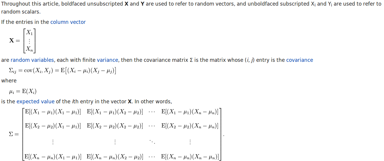
First, we should know how to calculate covariance matrix and correlation matrix.
According to the wikipedia page, we have the calculation procedure of covariance matrix as:
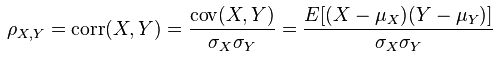
And the calculation procedure of correlation matrix is:
I am going to use an R example to illustrate the calculation procedures. Let’s say we have a `m1` matrix composed of six columns.
v1 <- c(1,1,1,1,1,1,1,1,1,1,3,3,3,3,3,4,5,6)
v2 <- c(1,2,1,1,1,1,2,1,2,1,3,4,3,3,3,4,6,5)
v3 <- c(3,3,3,3,3,1,1,1,1,1,1,1,1,1,1,5,4,6)
v4 <- c(3,3,4,3,3,1,1,2,1,1,1,1,2,1,1,5,6,4)
v5 <- c(1,1,1,1,1,3,3,3,3,3,1,1,1,1,1,6,4,5)
v6 <- c(1,1,1,2,1,3,3,3,4,3,1,1,1,2,1,6,5,4)
m1 <- cbind(v1,v2,v3,v4,v5,v6)
The covariance matrix of `m1` is:
> cov(m1)
         v1        v2       v3        v4       v5       v6
v1 2.535948 2.3071895 1.300654 1.0849673 1.183007 1.026144
v2 2.307190 2.3790850 1.013072 0.9934641 1.071895 1.052288
v3 1.300654 1.0130719 2.535948 2.2026144 1.300654 1.084967
v4 1.084967 0.9934641 2.202614 2.4869281 1.084967 1.075163
v5 1.183007 1.0718954 1.300654 1.0849673 2.535948 2.379085
v6 1.026144 1.0522876 1.084967 1.0751634 2.379085 2.486928
So, let’s look at `cov(m1)[1,1] = 2.535948` and `cov(m2)[1,2] = 2.3071895`:
# nrow(m1) is the number of data points.
> (v1-mean(v1)) %*% (v1 - mean(v1) )/ (nrow(m1) - 1)
         [,1]
[1,] 2.535948
> (v1-mean(v1)) %*% (v2 - mean(v2) )/ (nrow(m1) - 1)
        [,1]
[1,] 2.30719
The correlation matrix of `m1` is:
> cor(m1)
          v1        v2        v3        v4        v5        v6
v1 1.0000000 0.9393083 0.5128866 0.4320310 0.4664948 0.4086076
v2 0.9393083 1.0000000 0.4124441 0.4084281 0.4363925 0.4326113
v3 0.5128866 0.4124441 1.0000000 0.8770750 0.5128866 0.4320310
v4 0.4320310 0.4084281 0.8770750 1.0000000 0.4320310 0.4323259
v5 0.4664948 0.4363925 0.5128866 0.4320310 1.0000000 0.9473451
v6 0.4086076 0.4326113 0.4320310 0.4323259 0.9473451 1.0000000
`cor(m1)[1,1]=1.000` and `cor(m1)[1,2]=0.9393083`. Let’s see how they are calculated:
> (v1-mean(v1)) %*% (v1 - mean(v1) )/ (nrow(m1) - 1)/ (sd(v1) * sd(v1))
     [,1]
[1,]    1
> (v1-mean(v1)) %*% (v2 - mean(v2) )/ (nrow(m1) - 1)/ (sd(v1) * sd(v2))
          [,1]
[1,] 0.9393083
Update 07/15/2015. end.
————————————————————————————————————————————————-
现在就是这篇帖子的主题,PCA是什么?以及PCA和SVD的关系。
[gview file=”https://czxttkl.com/wp-content/uploads/2015/06/PCA-SVD-NNMF.pdf” height=”1000px” width=”700px”]
Two examples of visualizing PCA
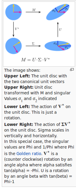
下图是一个SVD分解的示意图。每个矩阵都代表着一种空间的变化,那么M代表的变化可以分解为:
1. 先经过V这个旋转(Rotation)变化
2. 再经过$latex \Sigma$这个拉伸(Scaling)变化
3. 再经过U这个旋转(Rotation)变化
图中,起始的图形是一个半径为单位长度的圆形。
PCA, as visualized here, is trying to minimize the error between data and the principle component’s direction:

Update on 06/25/2015:
The following is a R script I wrote myself:

# A test file related to my post: https://czxttkl.com/?p=339
# and https://czxttkl.com/?p=397
remove(list=ls())
data("iris")
log.ir <- log(iris[,1:2])

# center but not scale by myself
log.ir[,1] <- log.ir[,1] - mean(log.ir[,1])
log.ir[,2] <- log.ir[,2] - mean(log.ir[,2])

ir.pca <- prcomp(log.ir, center = FALSE, scale. = FALSE)

# corresponds to p, x, y in my post.
p <- t(ir.pca$rotation)
x <- t(log.ir)
y <- p %*% x

# cov() calculates covariance matrix of the input matrix columns
# cov_y should have non-zero diaognal elements and close-to-zero non-diagonal elements
cov_y <- cov(t(y), t(y))

# Check if my calculation of covariance of y is consistent with cov_y
y_col2 <- t(y)[,2]
cov_y_2_2 <- (y_col2 %*% y_col2) / (length(y_col2) - 1)

# The red lines are the directions of principle component vectors. They should be orthogonal.
plot(log.ir, xlim=c(-1,1), ylim=c(-1,1))
points(t(y), col="blue")
abline(b=ir.pca$rotation[1,2]/ir.pca$rotation[1,1], a=0, col="red")
abline(b=ir.pca$rotation[2,2]/ir.pca$rotation[2,1], a=0, col="red")