czxttkl – Page 25

How to make match prediction using TrueSkill?

TrueSkill [1] is a widely accepted algorithm for matchmaking, in which player skills are initialized with a random variable following Gaussian distribution and then get updated through team-based match outcomes. Eventually, with sufficient amount of matches, player skill random variables will converge to some means with very small variance.

There are multiple open sourced libraries implementing the algorithm. For example, one in Python [2] and another in C# [3]. However in these open sourced libraries I don’t see how to predict new matches given learned player skill mean and variance.

Today I checked again the paper and other materials to assure that to predict a new match where draw is not allowed, whichever team has higher sum of means should be predicted to win. Why? Let’s use the example from the original TrueSkill paper.

In the factor graph above, we want to compare $latex t1$ vs $latex t2$ and $latex t2$ vs $latex t3$. Let’s take the comparison between t1 and t2 for example. We are essentially comparing $latex p1$ vs $latex p2+p3$. $latex s_1 \sim \mathcal{N}(\mu_1, \sigma_1^2)$ and $latex p_1 \sim \mathcal{N}(s_1, \beta^2)$. To get the distribution of $latex p_1$, we have:

$latex \int_{-\infty}^{\infty} \frac{1}{\sigma_1 \sqrt{2\pi}} e^{-\frac{(s_1 – \mu_1)}{2 \sigma_1^2}} \frac{1}{\beta \sqrt{2\pi}} e^{-\frac{(p_1 – s_1)}{2 \beta^2}} ds= \frac{1}{\sqrt{\sigma_1^2 + \beta^2} \sqrt{2\pi}} e^{- \frac{(p_1 – \mu_1)^2}{2(\sigma_1^2+\beta^2)}} &s=2$

Therefore $latex p_1$ is another random variable following normal distribution. $latex p_2$ and $latex p_3$ can be derived to be random variables in a similar fashion. Since we know that add/substract multiple normal random variables will result in a random variable with the mean equal to add/substract of the means of participating variables, we conclude that the predicted outcome between two teams relies on whether the sum of means of one team is greater than that of the other team. In our example, $latex d_1 \sim \mathcal{N}(\mu_1 – \mu_2 – \mu_3, \sigma’)$ for some $latex \sigma’$ not important to know for prediction.

if you want to know the winning probability of a player over another, checkout [5] and [6]

[1] http://research.microsoft.com/en-us/projects/trueskill/

[2] http://trueskill.org/

[3] http://www.moserware.com/2010/03/computing-your-skill.html

[4] http://www.tina-vision.net/docs/memos/2003-003.pdf

[5] http://stackoverflow.com/questions/28031698/with-the-trueskill-algorithm-given-two-players-ratings-how-can-i-calculate-th

[6] https://github.com/sublee/trueskill/issues/1#issuecomment-10491635

Optimization Overview

In this post, I am summarizing all I know for optimization. It is a hard, primary problem once you define your model with some kind of objective function integrating a bunch of parameters and you start to wonder how you could learn the values of those parameters to minimize (or maximize) the objective function.

Unconstrained Optimization

You wish to learn parameters to minimize the objective function and those parameters don’t have any constraints. If this is a convex problem, then there must be a global minimum and you can find it by finding all points whose first-order derivatives are zero. If the objective function is not convex, don’t panic. Gradient Descent (with lots of its variants such as momentum gradient descent, stochastic gradient descent, AdaGra) definitely help you to reach local minimum. People find that when the number of variables is large you will reach a not too bad local minimum. (missing reference here). Another family of approach is called quasi-Newton method which is my favorite. They have comparably fast speed as Newton Method does but its computation is way more economic. I implemented one unconstrained LBFGS algorithm in Python and some of its details are revealed here: https://czxttkl.com/?p=1257

Constrained Optimization

When it comes to constrained optimization, there exist tons of approaches which can be applied in different conditions. Here is a summary of techniques you can equip: (from https://ipvs.informatik.uni-stuttgart.de/mlr/marc/teaching/13-Optimization/03-constrainedOpt.pdf):

First of all, let’s get familiar with the foundations of constrained optimization.

Suppose we are faced a constrained optimization problem:

$\min\limits_{x \in \mathbb{R}^n} f(x)$

s.t. $c_i(x)=0, i \in \xi$ and $g_i(x) \geq 0, i \in \iota$

At a feasible point $x$ , the inequality constraint $i \in \iota$ is said to be active if $g_i(x)=0$ and inactive if the strict inequality $g_i(x) > 0$ is satisfied.

The active set $\mathcal{A}(x)$ at any feasible $x$ consists of the equality constraint indices from $\xi$ together with the indices of the inequality constraints $i$ for which $g_i(x)=0$ , i.e., $\mathcal{A}(x)=\{i \in \xi\} \cup \{i \in \iota|g_i(x)=0\}$

LICQ: Given the point $x$ and the active set $\mathcal{A}(x)$ , we say that the linear independence constraint qualification (LICQ) holds if the set of the active constraint gradient $\{\nabla g_i(x), i \in \mathcal{A}(x)\}$ is linearly independent.

KTT (Karush-Kuhn-Tucker) conditions

KTT conditions are necessary conditions for a optimum solution in nonlinear programming. (Some of the constraints or the objective function is non-linear.) In other words, if a solution $x^*$ is a local minimum of a function $f$ which we aims to minimize under certain equality constraints $\{c_i(x) | i \in \xi \}$ and inequality constraints $\{g_i(x) | i \in \iota\}$ , then $x^*$ , $f(x^*)$ , $\{h_i(x^*)\}$ and $\{c_i(x^*)\}$ must satisfy KTT conditions. The reverse, i.e., if a solution $x$ satisfies KTT conditions then it is a local minimum, is not always true.

More formally to state KTT conditions:

Assume $x^*$ is a local solution which achieves local minimum of $f(x)$ . If $f(x)$ , $\{c_i(x) | i \in \xi\}$ and $\{g_i(x) | i \in \iota \}$ are continuously differentiable, and LICQ holds at $x^*$ , then there is a Lagrange multiplier vector $\lambda^*$ , with components $\lambda_i^*, i \in \xi \cup \iota$ , such that following conditions are satisfied at $(x^*, \lambda^*)$ :

Define: $\mathcal{L}(x, \lambda) = f(x) - \sum\limits_{i \in \xi} \lambda_i c_i(x) - \sum\limits_{i \in \iota} \lambda_i g_i(x)$
$\nabla \mathcal{L}(x^*, \lambda^*)=\nabla f(x^*) - \sum\limits_{i \in \xi} \lambda_i^* \nabla c_i(x^*) - \sum\limits_{i \in \iota | g_i(x^*)=0} \lambda_i^* \nabla g_i(x^*)= 0$
$c_i(x^*) = 0, i \in \xi$
$g_i(x^*) \geq 0, i \in \iota$
$\lambda_i^* \geq 0, i \in \iota$
$\lambda_i^* c_i(x^*)=0, i \in \xi$
$\lambda_i^* g_i(x^*)=0, i \in \iota$

In $\nabla \mathcal{L}(x^*, \lambda^*)$ , we ignore to subtract $\sum\limits_{i \in \xi \cup \iota \backslash \mathcal{A}(x^*)} \lambda_i^* \nabla c_i(x^*)$ because KKT conditions indicate that $\lambda_i=0$ for $i \in \xi \cup \iota \backslash \mathcal{A}(x^*)$ , i.e., for those inactive inequality constraints $g_i(x^*) > 0$ .

Note that, we require LICQ holds at $x^*$ so that $\lambda^*$ is unique. LICQ is called constraint qualification. There are other constraint qualifications that must hold to guarantee KKT conditions hold if $x$ is a local minimum. (See https://www.math.washington.edu/~burke/crs/516/notes/cq_lec.pdf) For example, if $x^*$ is a local minimum and Abadie constraint qualification (ACQ) holds at $x^*$ , then KTT conditions still hold. Here ACQ is a weaker constraint qualification than LICQ because LICQ => ACQ.

Here is my rough understanding of KKT conditions: We want to let $argmin_x \mathcal{L}(x, \lambda) = argmin_x f(x)$ subject to the same constraints. $\mathcal{L}(x, \lambda)$ consists of $f(x)$ and a bunch of $-\lambda_i g_i(x)$ and $-\lambda_i c_i(x)$ . To make sure $\mathcal{L}(x, \lambda)$ and $f(x)$ have the same local solution $x^*$ , you must do the following checks:

For a local minimum $x^*$ of $f(x)$ , if $\lambda_i^* g_i(x^*) > 0$ , then $argmin_x \mathcal{L}(x, \lambda) = argmin_x f(x)$ is not guaranteed unless $\lambda_i^* g_i(x^*) = 0$ . Put it in other words, if you want $\mathcal{L}(x, \lambda)$ to have the same optimum as $f(x)$ , then $\lambda_i g_i(x)$ , the term added to $\mathcal{L}(x, \lambda)$ besides $f(x)$ , should not influence $f(x)$ and $\mathcal{L}(x, \lambda)$ to reach their local minimum at $x^*$ at the same time.
For equality constraints and active inequality constraints, $\lambda_i^* c_i(x^*)$ and $\lambda_i^* g_i(x^*)$ are zeros which can be safely added to $\mathcal{L}(x^*, \lambda^*)$ without affecting $x^*$ being the local optimum for both $\mathcal{L}(x, \lambda)$ and $f(x)$ .

Next, you should note that for the local minimum $x^*$ , $\nabla f(x^*) - \sum\limits_{i \in \xi} \lambda_i^* \nabla c_i(x^*) - \sum\limits_{i \in \iota | g_i(x^*)=0} \lambda_i^* \nabla g_i(x^*)= 0$ . This means, at $x^*$ , the force to minimize $f(x)$ is pulled by the force to ensure $x^*$ to stay in feasible areas. This can be illustrated in the following example:

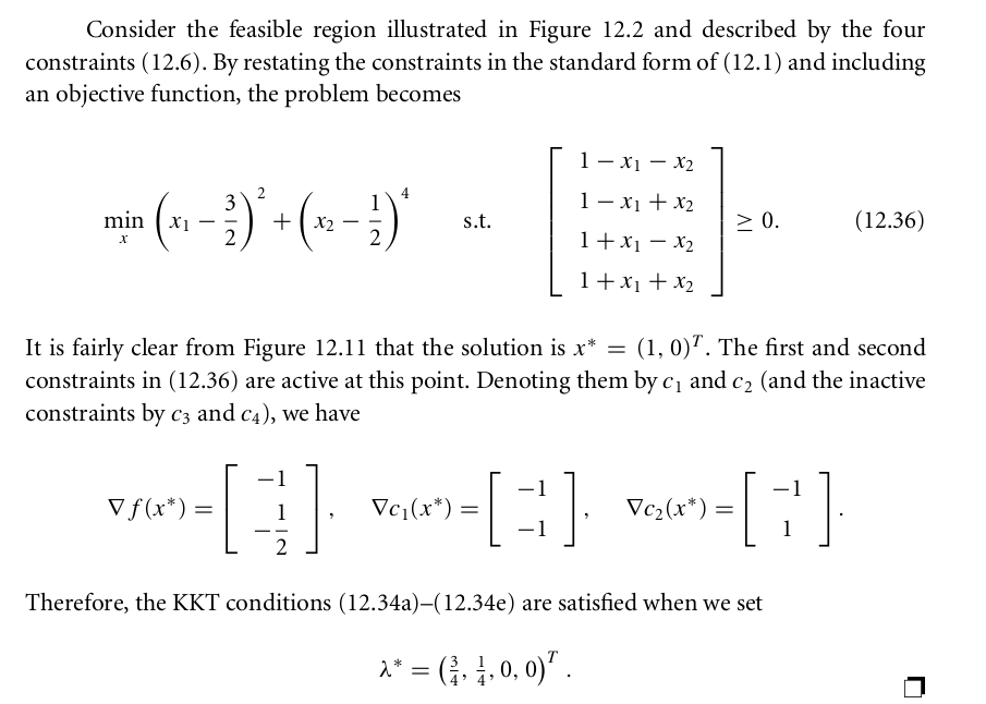
As you can see, at $x^*=(1, 0)$ , the force to minimize $f(x)$ is the direction $-\nabla f(x^*) = (-1, -\frac{1}{2})$ (marked as purple arrow) . The force to pull $x^*$ to stay the feasible region (the square in the middle) is $\nabla c_1(x^*)$ and $\nabla c_2(x^*)$ (marked as red arrows). $\lambda^*=(\frac{3}{4}, \frac{1}{4}, 0, 0)$ makes sure $\nabla f(x^*)$ , $\nabla c_1(x^*)$ and $\nabla c_2(x^*)$ are linearly dependent at this point so that $x*$ can’t be dragged any further by any force.

Although knowing a feasible point $x$ and a $\lambda$ satisfying KTT conditions is generally not sufficient to conclude $x$ is the solution for the constrained optimization problem, under certain conditions $x$ indeed is the solution. For example, if you know additional information like Second Order Sufficient Conditions, then KTT conditions become sufficient to say $x$ is a local solution. For another example, if Slater’s condition holds for the constrained problem, then $(x, \lambda) \text{ satisfy KTT conditions } \Rightarrow x \text{ is a local solution}$ . (Ref: http://math.stackexchange.com/questions/379543/kkt-and-slaters-condition, https://www.cs.cmu.edu/~ggordon/10725-F12/slides/16-kkt.pdf p11). In the famous SVM model, the objective function and its constraints also satisfies Slater’s condition such that KTT conditions are sufficient and necessary. See https://czxttkl.com/?p=3114 for how we do optimization for SVM using KTT.

Actually, Slater’s condition is originally used to prove that the strong duality holds for the constrained problem. Let’s illustrate it by introducing Duality Theory.

Duality Theory

An optimization problem can usually be constructed as a primal problem, for which there exists a corresponding dual problem. The dual problem sometimes has magics such that the computation of the dual problem is easier, or the solution of the dual problem can hint bounds of the primal problem.

Let’s say we face the same optimization problem as follows.

$\min\limits_{x \in \mathbb{R}^n} f(x)$

s.t. $c_i(x)=0, i \in \xi$ and $g_i(x) \geq 0, i \in \iota$

This problem can be converted into a primal problem incorporating all the constraints $c_i(x)=0, i \in \xi$ and $g_i(x) \geq 0, i \in \iota$ :

$\min\limits_x p(x) = \min\limits_x \max\limits_{\lambda} \mathcal{L}(x, \lambda) = \min\limits_x \max\limits_{\lambda} f(x) - \sum\limits_{i \in \xi} \lambda_i c_i(x) - \sum\limits_{i \in \iota} g_i(x)$ subject to $\lambda \geq 0$

Why does the primal problem look like this? This is because the minimum of $p(x)$ is the same as the minimum of the original constrained optimization problem. For those $x$ s.t. $c_i(x) \neq 0 \text{ or } g_i(x) <0$ , $\max\limits_{\lambda} \mathcal{L}(x, \lambda) = \infty$ therefore any $x$ violating the constraints is definitely not the solution to the primal problem. For those $x$ satisfying the constraints, $\max\limits_{\lambda} \mathcal{L}(x, \lambda) =f(x)$ . Therefore, it is equivalent to $\min\limits_x p(x)$ as to do the original constrained problem.

Now we construct the dual problem of the primal problem. The dual problem is:

$\max\limits_{\lambda \in \mathbb{R}^{|\xi \cup \iota|}} q(\lambda) = \max\limits_{\lambda} \inf\limits_x \mathcal{L}(x, \lambda)$ subject to $\lambda \geq 0$ . (Here $\inf h(x)$ is infimum function denoting the lower bound of $h(x)$ . For example, $\inf\limits_x e^{-x} = 0$ . We don’t use $\min\limits_x h(x)$ to denote the lower bound of $h(x)$ because $h(x)$ can be infinitely close to but never reach the lower bound for any $x$ .)

Now we have Weak Duality which goes like this:

$\max\limits_{\lambda} q(\lambda) = \max\limits_{\lambda} \inf\limits_x \mathcal{L}(x, \lambda) \leq \min\limits_x p(x) = \min\limits_x \max\limits_{\lambda} \mathcal{L} (x, \lambda)$ for any $\lambda \geq 0$ and any feasible $x$

This suggests that the optimum of the dual problem has some non-negative duality gap smaller than the optimum of the primal problem. If we can close the duality gap between the dual and the primal, we can solve the primal problem by solving the dual problem which sometimes is much easier. The duality gap is zero when Strong Duality holds for the optimization problem.

Ref: http://jackvalmadre.tumblr.com/post/15798388985

Here for the duality theory for linear programming specifically: https://www.math.washington.edu/~burke/crs/407/notes/section4.pdf

Lagrange Multiplier

Lagrange Multiplier is used for finding minimum/maximum of a function under equality constraints. Lagrange Multiplier utilizes an important fact that when a function achieves a minimum/maximum under certain equality constraints, the gradient of the function and the gradients of the constraints have the same direction. What Lagrange Multiplier essentially does is to add constraints, each multiplied by a Lagrange Multiplier, to the objective function to form an “auxiliary objective function”. By taking the derivative of the auxiliary objective function and set it to zero, we can find all stationary points of the auxiliary objective function. Among those stationary points, there must be at least one that achieves the minimum/maximum. A good tutorial of Lagrange Multiplier can be found here: http://www.slimy.com/~steuard/teaching/tutorials/Lagrange.html

Lagrange Multiplier method can be modified to solve constrained problems with inequality constraints. The multiplier and optimal solution can be found by using KKT conditions: http://www.csc.kth.se/utbildning/kth/kurser/DD3364/Lectures/KKT.pdf. One example of using Lagrange Multiplier to solve problems with inequality constraints can be found here: http://users.wpi.edu/~pwdavis/Courses/MA1024B10/1024_Lagrange_multipliers.pdf.

A family of constrained problem solvers converts constrained problems into unconstrained problems. In the family of such solvers, one kind of algorithms are called inexact method: the solution to the transformed unconstrained problem is close but not exactly the same to that to the original constrained problem. The other kind of algorithm is called exact method in which the solution does not change after the transformation. In the following introduced algorithms, Quadratic Penalty Method belongs to inexact method. $\ell_1$ Penalty Method and Augmented Lagrangian Method belong to exact method.

Quadratic Penalty Method

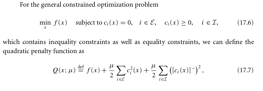
$\ell_1$ Penalty Method

When only equality constraints are present, $Q(x;\mu)$ is smooth. But when inequality constraints are also present, $Q(x;\mu)$ is not smooth any more. Moreover, $\mu$ sometimes goes to be very large in iterations, likely to cause the Hessian matrix of $Q(x;\mu)$ , $\nabla_{xx}^2 Q(x;\mu)$ , become ill-conditioned.

$\ell_1$ Penalty Method

$\ell_1$ Penalty Method is exact but the non-smoothness of $\phi_1(x;\mu)$ makes it difficult to find minimizer of it. Refer to the textbook to some hack ways to solve it.

Augmented Lagrangian Method

It reduces the possibility of ill-conditioning of Quadratic Penalty Method and preserves the smoothness as opposed to $\ell_1$ Penalty Method.

https://en.wikipedia.org/wiki/Augmented_Lagrangian_method

Stochastic Gradient Descent

Stochastic Gradient Descent has been popular among large-scale machine learning. So far the most canonical text about stochastic gradient descent I’ve found is: Bottou, L. (2012). Stochastic gradient descent tricks. In Neural Networks: Tricks of the Trade (pp. 421-436). Springer Berlin Heidelberg.

The core idea is that “use stochastic gradient descent when training time is the bottleneck“. What does this mean? Roughly understanding, gradient descent should result in higher training accuracy than its stochastic counterpart because the former uses the full dataset to calculate a less noisy weight update. However in an iteration, gradient descent will take a long time to traverse all samples to calculate weight update. During that, the weight update of stochastic gradient descent has happened many times and the objective function it optimizes has been improved many times! Therefore, the paper points out that “SGD needs less time than the other algorithms to reach a predefined expected risk”. Please understand Table 2 in the paper carefully.

Projected Gradient Descent

This post highly summarizes the difference between ordinary gradient descent and projected gradient descent: http://math.stackexchange.com/questions/571068/what-is-the-difference-between-projected-gradient-descent-and-ordinary-gradient

This paper showcases how to use projected gradient descent for non-negative matrix factorization:

Lin, C. J. (2007). Projected gradient methods for nonnegative matrix factorization. Neural computation, 19(10), 2756-2779.

This paper also points out that if all the constraints are just non-negativity constraint, then we can set parameters $P=P'^2$ , then we can just optimize the objective w.r.t $P'$ , where $P' \in \mathbb{R}$ .

However, I have not seen projected stochastic gradient descent been applied on any problem. I will keep searching why it is rarely used. My guess is that stochastic-based updates are already very noisy and unstable. The projection performed after each stochastic update will make parameter updates even more unstable such that the optimization cannot find the correct path towards the optimal parameterization.

Quadratic Programming

Quadratic Programming is an optimization problem with a quadratic objective function and linear constraints. If constraints only consist of equalities, it looks like the following:

$\min_x q(x) = \frac{1}{2} x^T G x + x^T c \\ \text{subject to } Ax=b, A \in \mathbb{R}^{m \times n}, m < n$

Now we introduce an iterative way to solve the quadratic programming with equality constraints, which is covered in Chapter 16.3 of Numerical Optimization by Nocedal & Wright.

First, the optimal solution $x^* \in \mathbb{R}^n$ can be represented as $x^*=Yx_Y+Zx_Z$ , where $x_Z \in \mathbb{R}^{n-m}$ , $x_Y \in \mathbb{R}^{m}$ , $Y \in \mathbb{R}^{n \times m}$ , $Z \in \mathbb{R}^{n \times (n-m)}$ and $AZ=0$ . Note that in $x^*=Yx_Y+Zx_Z$ , $Y$ , $Z$ and $x_Y$ are some constants determined by elimination algorithms (introduced soon). $x_Z$ is the free variables that $\in \mathbb{R}^{n-m}$ . Why can $x$ be represented by $x_Z$ ? This is because $A$ has rank $m$ ( $m<n$ ) therefore we can use $n-m$ variables in $x_Z$ to represent $n$ variables in $x$ . Since $AZ=0$ , $Ax=b$ indicates that $AYx_Y=b$ . Therefore, $Yx_Y$ is a solution satisfying $Ax=b$ . Therefore, $x^*=Yx_Y+Zx_Z$ can be seen as a sum of a particular solution to the constraint $Ax=b$ (the first term) plus a transformation $Z$ applied on $x_Z$ . Since $AZ=0$ holds, any choice of $x_Z$ will still satisfy the constraint $Ax=b$ . The only difference of choices of $x_Z$ remains to be whether $x_Z$ minimizes the objective function.

To determine $Y$ , $Z$ and $x_Y$ , we use methods called simple elimination or general elimination:

1. simple elimination says that: find a permutation matrix $P$ such that $AP= [B|N]$ . Here the columns of $B \in \mathbb{R}^{m \times m}$ are a subset of columns of $A$ that are linearly independent. $N \in \mathbb{R}^{m \times (n-m)}$ . Now that if we set:

, $x$ can be represented as $x = Yb + Zx_Z$ .

2. general elimination uses QR-factorization on $A^T\Pi$ ( $\Pi$ is a permutation matrix to obtain $Q_1$ , $Q_2$ and $R$ :

Then, set $x$ to

(I am unclear of when to use simple elimination or general elimination as the book compares the two algorithms vaguely to me. )

Now let’s go back solving the quadratic programming problem once obtaining $x^*=Yx_Y+Zx_Z$ . Plugging it to $\min_z q(x)=\frac{1}{2} x^T G x + x^T c$ with all constants removed, we obtain $min_{X_z} \frac{1}{2}x_Z^T Z^T G Z x_Z + x_Z^T (Z^T G Y x_Y + Z^T c)$ . The textbook gives an iterative method to find desired $x_Z$ using Conjugate Gradient method, with the assumption that $Z^T G Z$ is positive definite:

$\ell_1$ regularization

Please note that $\ell_1$ regularization refers to the problem of the form: $\min\limits_x f(x) = L(x) + \lambda \left\Vert x\right\Vert_1$ . Such forms of problems often have solutions $x^*$ with great sparsity. That is why $\ell_1$ regularization is often used to achieve feature selection. This kind of problem is different to another kind of problem (also introduced in this post): use $\ell_1$ as nonsmooth exact penalty function to solve constrained problems.

This paper gives a full overview of methods to solve $\ell_1$ regularization problems. I am here giving a simple approach:

When given a $\ell_1$ regularization problem $\min\limits_{x \in \mathbb{R}^n} f(x) = L(x) + \lambda \left\Vert x\right\Vert_1$ , we can write an equivalent constrained optimization problem: $\min\limits_{x^+,x^-} L(x^+ - x^-) + \lambda(x^+ + x^-)\quad s.t. \quad x^+ = \max(0,x), x^- = -\min(0,x), x^+ \geq 0, x^- \geq 0$

To explain why we can write such equivalent constrained optimization problem, let’s first check that $x^+ - x^- = x$ and $x^+ + x^- = |x|$ . Therefore $L(x^+ - x^-)=L(x)$ and $\lambda(x^+ + x^-) = \lambda\left\Vert x\right\Vert_1$ . Depending on the strength of $\lambda$ , $x^+$ and $x^-$ will be constrained to not fluctuate too radically, resulting the constrained $\ell_1$ norm of original $x$ . Eventually, the $\ell_1$ regularization problem becomes a box constraint optimization problem (albeit the box is single side bounded, because you only require $x^+$ and $x^-$ to be non-negative.)

There is an online implementation of such method using L-BFGS-B (box constraint of L-BFGS): https://gist.github.com/vene/fab06038a00309569cdd

Coordinate Descent

https://www.cs.cmu.edu/~ggordon/10725-F12/slides/25-coord-desc.pdf

Some Topics to Explore

Non convex global optimization: http://mathoverflow.net/questions/32533/is-all-non-convex-optimization-heuristic

Leetcode 202: Happy Number

https://leetcode.com/problems/happy-number/

Write an algorithm to determine if a number is “happy”.

A happy number is a number defined by the following process: Starting with any positive integer, replace the number by the sum of the squares of its digits, and repeat the process until the number equals 1 (where it will stay), or it loops endlessly in a cycle which does not include 1. Those numbers for which this process ends in 1 are happy numbers.

Example: 19 is a happy number

1² + 9² = 82
8² + 2² = 68
6² + 8² = 100
1² + 0² + 0² = 1

Code

class Solution(object):
    def isHappy(self, n):
        """
        :type n: int
        :rtype: bool
        """
        if n <= 0:
            return False
        
        nums = set()
        
        while True:
            n = sum([int(d)**2 for d in str(n)])
            if n == 1:
                return True
            if n in nums:
                return False
            nums.add(n)

Idea

A number if happy if it has 1 in its happy loop. If a number is unhappy, it will endless loop, meaning at some point the square sum of digits will have repeated values. In my code, I am using a set to record the square sum in the loop. Whenever we see repeated square sum, we return unhappy. Of course, this method requires O(N) space, where N is the size of digits of the given number.

Another method is to use the idea of Floyd Cycle Detection algorithm: create a fast and a slow pointer. If fast pointer has the same value as the slow pointer, there must be a cycle. If the point they meet has the value, the number is happy.

int digitSquareSum(int n) {
    int sum = 0, tmp;
    while (n) {
        tmp = n % 10;
        sum += tmp * tmp;
        n /= 10;
    }
    return sum;
}

bool isHappy(int n) {
    int slow, fast;
    slow = fast = n;
    do {
        slow = digitSquareSum(slow);
        fast = digitSquareSum(fast);
        fast = digitSquareSum(fast);
    } while(slow != fast);
    if (slow == 1) return 1;
    else return 0;
}

Refs: https://leetcode.com/discuss/33055/my-solution-in-c-o-1-space-and-no-magic-math-property-involved

Leetcode 143: Reorder List

https://leetcode.com/problems/reorder-list/

Given a singly linked list L: L₀→L₁→…→L_n-1→L_n,
reorder it to: L₀→L_n→L₁→L_n-1→L₂→L_n-2→…

You must do this in-place without altering the nodes’ values.

For example,
Given {1,2,3,4}, reorder it to {1,4,2,3}.

Code

# Definition for singly-linked list.
# class ListNode(object):
#     def __init__(self, x):
#         self.val = x
#         self.next = None

class Solution(object):
    def reorderList(self, head):
        """
        :type head: ListNode
        :rtype: void Do not return anything, modify head in-place instead.
        """
        if not head or not head.next:
            return 
        
        # find the middle point, where p1 will finally land.
        p1 = p2 = head        # p1: fast pointer, p2: slow pointer
        while p2.next and p2.next.next:
            p2 = p2.next.next
            p1 = p1.next
        
        p3 = p1.next
        head2 = None
        p1.next = None
        
        # reverse the latter part
        while p3:
            next = p3.next
            p3.next = head2
            head2 = p3
            p3 = next
        
        # the first part has at least one more element than the second part
        while head:
            next1 = head.next
            head.next = head2
            if head2:
                next2 = head2.next
                head2.next = next1
            head = next1
            head2 = next2

Idea

There are three steps:

use a slow pointer and a fast pointer to find the middle point of the linked list. The middle point will split the linked list into two parts.
Reverse the second part of the linked list.
Merge the two parts.

Leetcode 166: Fraction to Recurring Decimal

https://leetcode.com/problems/fraction-to-recurring-decimal/

Given two integers representing the numerator and denominator of a fraction, return the fraction in string format.

If the fractional part is repeating, enclose the repeating part in parentheses.

For example,

Given numerator = 1, denominator = 2, return “0.5”.
Given numerator = 2, denominator = 1, return “2”.
Given numerator = 2, denominator = 3, return “0.(6)”.

Code

class Solution(object):
    def fractionToDecimal(self, numerator, denominator):
        """
        :type numerator: int
        :type denominator: int
        :rtype: str
        """
        if numerator == 0:
            return "0"
            
        res = ''
        if (numerator < 0) ^ (denominator < 0): # if either or numerator or denominator is negative
            res += "-"
            
        numerator, denominator = abs(numerator), abs(denominator)
            
        quot = numerator / denominator
        res += str(quot)    
        rem = numerator % denominator
        if rem == 0:
            return res
        
        res += "."
        rems = {}     # key is the last remainder and the value is the length of the result
                      # after filled with the quotient of the last remainder * 10 / denominator
        while True:
            rem_new = rem * 10
            quot = rem_new / denominator
            rem_new = rem_new % denominator
            
            if rem_new == 0:
                return res + str(quot) 
                
            if rems.get(rem):
                idx = rems.get(rem)-1
                return res[:idx] + "(" + res[idx:] + ")"
            
            res += str(quot)
            rems[rem] = len(res)
            rem = rem_new

Idea

We use the basic idea of division to calculate every digit of the result. Besides many corner cases to be considered, the most difficult part is to determine if there is any recurrent part in the result:

I use a dictionary, `rems`, where key is the last remainder and the value is the length of the result after filled with the quotient of the last remainder * 10 / denominator. For example, given numerator=1 and denominator=6, the first digit after the decimal point is 1, which is the quotient of 1*10 by the denominator 6. At this time, we store (1, 3) in `rems` because 1 is the last remainder and 3 is the length of “0.1”. After generating the first digit, we have 4 as the remainder.

The second digit after the decimal point is 6. At this time, we add (4, 4) to `rems` due to the same manner. When we compute the next digit (the third digit after the decimal point), `rem` has set to the last remainder 4. `rem` is checked to be already a key in `rems` (line 34), we conclude we will start to get recurrent quotient(s). Therefore, we start to add parenthesis and output the result.

Leetcode 87: Scramble String

https://leetcode.com/problems/scramble-string/

Given a string s1, we may represent it as a binary tree by partitioning it to two non-empty substrings recursively.

Below is one possible representation of s1 = "great":

    great
   /    \
  gr    eat
 / \    /  \
g   r  e   at
           / \
          a   t

To scramble the string, we may choose any non-leaf node and swap its two children.

For example, if we choose the node "gr" and swap its two children, it produces a scrambled string "rgeat".

    rgeat
   /    \
  rg    eat
 / \    /  \
r   g  e   at
           / \
          a   t

We say that "rgeat" is a scrambled string of "great".

Similarly, if we continue to swap the children of nodes "eat" and "at", it produces a scrambled string "rgtae".

    rgtae
   /    \
  rg    tae
 / \    /  \
r   g  ta  e
       / \
      t   a

We say that "rgtae" is a scrambled string of "great".

Given two strings s1 and s2 of the same length, determine if s2 is a scrambled string of s1.

Code

class Solution(object):
    def isScramble(self, s1, s2):
        """
        :type s1: str
        :type s2: str
        :rtype: bool
        """
        if len(s1) != len(s2):
            return False
        elif not s1:
            return True
        
        n = len(s1)
        res = [[[False for _ in xrange(n)] for _ in xrange(n)] for _ in xrange(n+1)]  # the size of the first dim is n+1
                                                                                      # easy for indexing
        for j in xrange(n):
            for m in xrange(n):
                res[1][j][m] = (s1[j] == s2[m])
            
        for i in xrange(2, n+1):
            for j in xrange(n-i+1):
                for m in xrange(n-i+1):
                    for k in xrange(1,i):
                        res[i][j][m] |= (res[k][j][m] and res[i-k][j+k][m+k]) \
                                        or (res[k][j][m+i-k] and res[i-k][j+k][m])
                        
        return res[n][0][0]

Idea

See here: http://tianmaying.com/tutorial/LC87

One note is that we put for i in xrange(2, n+1) at the outmost loop (line 20), where `i` is the length of the two substrings, `s1[j:j+i] and s2[m:m+i]`, under comparison. When we calculate `res[i][j][m]`, we always need some `res[k’][j’][m’]` where `k’ < i`. Therefore, we need to calculate `res` in ascending order of `i`, the first dimension of `res`.

Leetcode 147: Insertion Sort List

https://leetcode.com/problems/insertion-sort-list/

Sort a linked list using insertion sort.

Code

# Definition for singly-linked list.
# class ListNode(object):
#     def __init__(self, x):
#         self.val = x
#         self.next = None

class Solution(object):
    def insertionSortList(self, head):
        """
        :type head: ListNode
        :rtype: ListNode
        """
        new_head = ListNode(0)
        cur = head
        while cur:
            isrt = new_head
            next = cur.next
            
            while isrt.next and isrt.next.val < cur.val:
                isrt = isrt.next
            
            cur.next = isrt.next
            isrt.next = cur
            cur = next
            
        return new_head

Idea

By definition, insertion sort is inserting each element to the current sorted array by comparing it to the elements in the current sorted array. It requires O(N^2) time asymptotically. In my code, `isrt` is used to locate the correct position to insert the new element. It is set to the head every time a new element needs to be inserted (Line 16).

However, the code above can’t pass the leetcode OJ. One way to circumvent it is to set `isrt` more passively (set `isrt` only when very necessary) instead of setting it to head for every new element to be inserted.

# Definition for singly-linked list.
# class ListNode(object):
#     def __init__(self, x):
#         self.val = x
#         self.next = None

class Solution(object):
    def insertionSortList(self, head):
        """
        :type head: ListNode
        :rtype: ListNode
        """
        new_head = ListNode(0)
        cur = head
        isrt = new_head
        
        while cur:
            next = cur.next
            
            if not isrt or not isrt.next or isrt.next.val>=cur.val:
                isrt = new_head
            
            while isrt.next and isrt.next.val < cur.val:
                isrt = isrt.next
            
            cur.next = isrt.next
            isrt.next = cur
            cur = next
            
            
        return new_head.next

Leetcode 6: ZigZag Conversion

https://leetcode.com/problems/zigzag-conversion/

The string "PAYPALISHIRING" is written in a zigzag pattern on a given number of rows like this: (you may want to display this pattern in a fixed font for better legibility)

P   A   H   N
A P L S I I G
Y   I   R

And then read line by line: "PAHNAPLSIIGYIR"

Write the code that will take a string and make this conversion given a number of rows:

string convert(string text, int nRows);

convert("PAYPALISHIRING", 3) should return "PAHNAPLSIIGYIR".

Code

class Solution(object):
    def convert(self, s, numRows):
        """
        :type s: str
        :type numRows: int
        :rtype: str
        """
        if s is None or len(s) <= numRows or numRows==1:
            return s
        
        res = ""
        for i in xrange(numRows):
            if i == 0 or i == (numRows-1):
                res += s[i::(2*numRows-2)]
            else:
                s1 = s[i::(2*numRows-2)]
                s2 = s[(2*numRows-2-i)::(2*numRows-2)]
                for c1, c2 in zip(s1, s2):
                    res += c1 + c2
                if len(s1) > len(s2):  # s1 is at most longer than s2 by one character
                    res += s1[-1]
        return res

Idea

Every `2*numRows-2` characters in `s` will form one zigzag. You can find the rules when outputing the zigzag horizontally:

Leetcode 164: Maximum Gap

https://leetcode.com/problems/maximum-gap/

Given an unsorted array, find the maximum difference between the successive elements in its sorted form.

Try to solve it in linear time/space.

Return 0 if the array contains less than 2 elements.

You may assume all elements in the array are non-negative integers and fit in the 32-bit signed integer range.

Code

import sys
import math

class Solution(object):
    def maximumGap(self, nums):
        """
        :type nums: List[int]
        :rtype: int
        """
        if not nums or len(nums) < 2:
            return 0
        
        # find max and min in nums
        max_num = -sys.maxint
        min_num = sys.maxint
        for i in nums:
            if i > max_num:
                max_num = i
            if i < min_num:
                min_num = i
        
        if max_num == min_num:
            return 0
        
        bucket_max = [None for _ in xrange(len(nums)+2)]  
        bucket_min = [None for _ in xrange(len(nums)+2)] 
        for i in nums:
            # max_num is actually assigned to n+2-th bucket  
            bucket = ((i-min_num) * (len(nums)+1)) / (max_num - min_num)  
            bucket_max[bucket] = max(bucket_max[bucket], i) if bucket_max[bucket] is not None else i
            bucket_min[bucket] = min(bucket_min[bucket], i) if bucket_min[bucket] is not None else i
        
        max_gap = 0
        prev_max = bucket_max[0]       # the first bucket must have one element
        for i in xrange(1, len(bucket_min)):
            if bucket_min[i] is not None:
                max_gap = max(bucket_min[i] - prev_max, max_gap)
                prev_max = bucket_max[i]
            
        return max_gap

Idea

This is a problem using the classic ideas of bucketing and pigeon hole principle. The logic is that, we create `n+1` buckets between `max_num` and `min_num`, where `max_num` and `min_num` of the array can be found in O(N) time. Since there are only `n` numbers in the array, there must be at least one bucket without any number landing in it. This important factor indicates that the max distance of two consecutive numbers in the sorted form must happen between the maximal number in one previous bucket and the minimal number in one latter bucket and the two buckets have at least one empty bucket between them. Any numbers falling into the same bucket will not have the difference exceeding the bucket range, which is `(max_num-min_num)/(n+1)`.

Leetcode 71: Simplify Path

https://leetcode.com/problems/simplify-path/

Given an absolute path for a file (Unix-style), simplify it.

For example,
path = "/home/", => "/home"
path = "/a/./b/../../c/", => "/c"

click to show corner cases.

Corner Cases:

Did you consider the case where path = "/../"?
In this case, you should return "/".
Another corner case is the path might contain multiple slashes '/' together, such as "/home//foo/".
In this case, you should ignore redundant slashes and return "/home/foo".

Code

class Solution(object):
    def simplifyPath(self, path):
        """
        :type path: str
        :rtype: str
        """
        paths = path.split("/")
        fs = []
        for p in paths:
            if p == "..":
                # when fs is empty, ".." has no effect
                if fs:
                    fs.pop()
            elif p == ".":
                pass
            elif p == "":
                pass
            else:
                fs.append(p)
        return "/" + "/".join(fs)

Idea

Since there could be “..” (the up level folder) and “.” (the current folder) in the path, it is natural to maintain a stack to record folder hierarchy. The crux of this problem is to consider all possible corner cases, such as paths with two or more consecutive backslashes, or paths ending with backslashes, or paths already landing in “/” but with more “..” followed.