In order to achieve a filter rule with OR operation, you must specify conditions connected by the keyword “OR” (must be in upper cases).
For example:

In order to achieve a filter rule with OR operation, you must specify conditions connected by the keyword “OR” (must be in upper cases).
For example:
If you do not have root privilege and want to install a python module, you can try the following approach:
python setup.py install --user
This will install packages into subdirectories of site.USER_BASE. To check what is the value of site.USER_BASE, use:
import site
print site.USER_BASE
reference: https://docs.python.org/2/install/
Update 2018/01/06:
using pip to install a python package:
pip install --user package_name
Embedding methods have been widely used in graph, network, NLP and recommendation system. In short, embedding methods vectorize entities under study by mapping them into a shared latent space. Once vectorized representation of entities are learned (through either supervised or unsupervised fashion), a lot of knowledge discovery work can be done: clustering based on entity vectors, analyze each dimension of the latent space, make recommendation, so on so forth.
When you learn embedding by supervised learning, you define a objective function that forges interaction of entity vectors and then learn vectors through maximizing/minimizing the objective function. When you learn embedding through unsupervised learning, you define how occurrences of data should conform to a conjured, underlying probability function in terms of entity vectors. This will be elaborated more in the following.
A widely known embedding method is matrix factorization in recommendation system. Affinity of a user and an item is often modeled as the dot product of the two corresponding entity vectors. When you are given a huge, sparse user-item matrix, you try to learn all user/item vectors such that their dot products can maximally approximate the entries in the sparse matrix. For more information, see [2]
Embedding in NLP has been rapidly developed recently. Let’s see a few classic embedding NLP models.
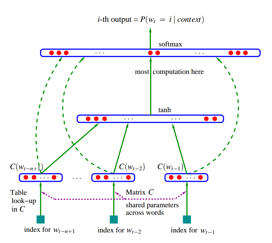
[3] published 2003. It tries to predict t-th word given t-1 words previously seen in word sequences. The model extends a neural network model:


 that indeed appears after
  :
: 

The diagram of the model structure (from the paper [3]):
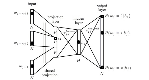
Equivalently, the model structure from [1]:
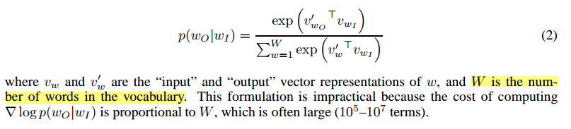
One problem is that in the normalization term in the softmax is expensive when vocabulary size is usually large. In [3], it proposes several parallelism implementation to accelerate learning. The other alternative is using hierarchical softmax [4, 5], which only needs to evaluate  for each softmax calculation. There are several other more efficient algorithms that are proposed to sidestep the calculation of softmax.
C&W model [17, 18]
C&W model has the following structure:
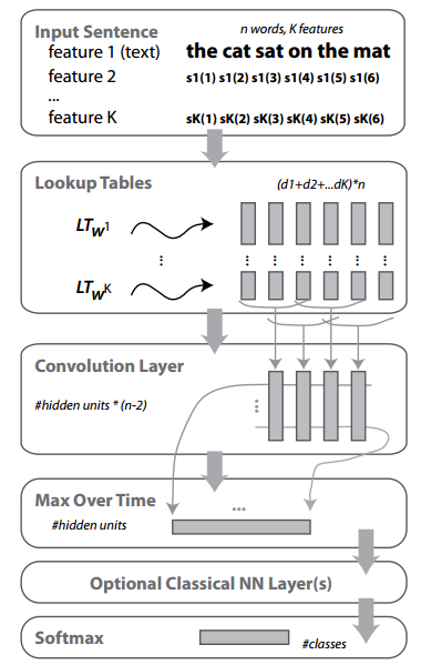
First, a word has multiple features (feature 1 ~ feature K), each has a  dimension embedding. Then a convolution layer is added to summarize surrounding embedding of each word. Then a max pooling is added so that most salient features will be kept. The last few layers are classic NN layers for supervised learning.
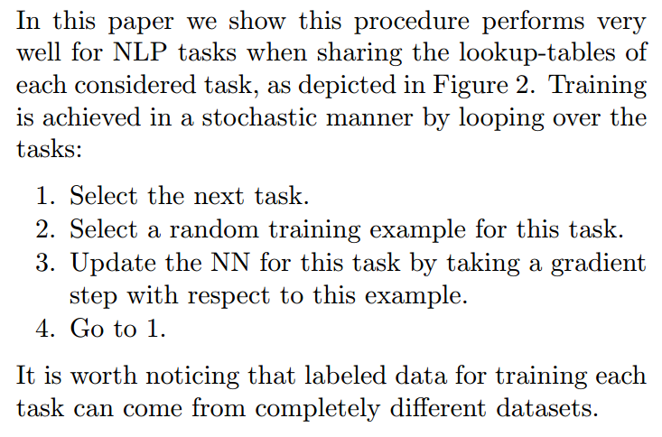
One contribution of the papers is to propose multi-task learning under the same, shared embedding table. The multi-task learning procedure is as follows:
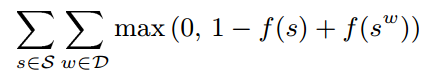
Furthermore, the tasks to be learned can be either supervised or unsupervised. In section 5 of [17], it introduces how to train a language model “to discriminate a two-class classification task”. Note the special ranking-type cost it uses:
Continuous bag-of-words [5]
This model is easy to understand. Projection layer is no longer the horizontal concatenation of word vectors [3]. Instead we just sum over all input word vectors as the input before the hidden layer.
Skip-gram [6]
Note to differentiate this with [7]. Instead of using a whole sequence to predict the right next word, Skip-gram uses one word to predict its every surrounding word. Specifically, the objective function is:

If in every pair of  , we denote
  as
as  and as
  , then we have
However, this objective function suffers the problem we described in [3]: the normalization term in softmax is expensive to calculate because vocabulary is often large. Therefore, they propose to use Negative sampling, which replaces  in the objective function above with:
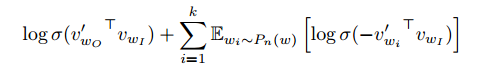
Since we are maximizing the objective function, we can understand it in such intuition: we want  as large as possible. Therefore,
  and
and  should be as similar as possible. On the other hand, the original normalization term in softmax can be seen to be replaced by
 ![\sum\limits_{i=1}^k \mathbb{E}_{w_i \sim P_n(w)}[\log\sigma({-v'_{w_i}}^T v_{w_I})]](https://czxttkl.com/wp-content/ql-cache/quicklatex.com-1cea7eb7c36b01e91574bbeffdafd7a6_l3.png "Rendered by QuickLaTeX.com") , which contains
, which contains  log-sigmoid function smoothing the negative dot products with noisy word vectors. Of course, to maximize it,
  and should be as dissimilar as possible.
Finally, the authors claim that using a modified unigram distribution  is good in practice. I guess the unigram distribution means each word has the probability mass correlated to the frequencies it appears in the data.
Miscellaneous NLP paper
The following are some papers with less attention so far.
[8] proposes that for each word, its word embedding should be unique across different supervised labels.
[9] proposes that adding more non-linear hidden layers could result in better differentiating ability in bag-of-word model.
For more NLP embedding overview, please see [1].
A heterogeneous network is a graph with multiple types of nodes and links can connect two different types of nodes. Meta-path define a series of links in a heterogeneous network [10, 11]. Heterogeneous network has richer information to harvest compared to single typed network.
[13] first learns embedding of documents, words, and labels. Then, classification .
[14] learns entity embedding (author, paper, keyword, etc) in bibliographical network for the author identification task. The objective function contains two parts: 1. task-specific embedding. author vector should be similar to paper vector which is obtained by averaging vectors per node type. 2. path-augmented heterogeneous network embedding. Two entity vectors should be similar if they are connected by certain meta-path.
[15] models normal events’ happening probabilities as interactions between entity embeddings.
[16] models people’s behavior on twitter to infer their political opinion embeddings. The behavior on twitter is converted to a heterogeneous network where there exist 3 types of links: follow, mention and retweet.
T-sne [12] is a dimensionality reduction technology with its goal to “preserve as much of the significant structure of the high dimensional data as possible in the low-dimensional map”. It focus on capturing the local structure of the high-dimensional data very well, while also revealing global structure such as the presence of clusters. To achieve that, t-sne converts pairwise similarity measurement to conditional probability and the objective function is the Kullback-Leibler divergence between conditional probability distribution under original high dimension and transformed low dimension space. It has been widely used for data interpretation in embedding papers.
[1] http://sebastianruder.com/word-embeddings-1/index.html
[2] https://czxttkl.com/?p=1214
[3] Bengio, Y., Ducharme, R., Vincent, P., & Jauvin, C. (2003). A neural probabilistic language model. journal of machine learning research, 3(Feb), 1137-1155.
[4] Morin, F., & Bengio, Y. (2005, January). Hierarchical Probabilistic Neural Network Language Model. In Aistats (Vol. 5, pp. 246-252).
[5] Mikolov, T., Chen, K., Corrado, G., & Dean, J. (2013). Efficient estimation of word representations in vector space. arXiv preprint arXiv:1301.3781.
[6] Mikolov, T., Sutskever, I., Chen, K., Corrado, G. S., & Dean, J. (2013). Distributed representations of words and phrases and their compositionality. In Advances in neural information processing systems (pp. 3111-3119).
[7] Li, C., N., Wang, B., Pavlu, V., & Aslam, J. Conditional Bernoulli Mixtures for Multi-Label Classification.
[8] Jin, P., Zhang, Y., Chen, X., & Xia, Y. (2016). Bag-of-Embeddings for Text Classification. In International Joint Conference on Artificial Intelligence (No. 25, pp. 2824-2830).
[9] Iyyer, M., Manjunatha, V., Boyd-Graber, J., & Daumé III, H. (2015). Deep unordered composition rivals syntactic methods for text classification. In Proceedings of the Association for Computational Linguistics.
[10] Kong, X., Yu, P. S., Ding, Y., & Wild, D. J. (2012, October). Meta path-based collective classification in heterogeneous information networks. In Proceedings of the 21st ACM international conference on Information and knowledge management (pp. 1567-1571). ACM.
[11] Sun, Y., Han, J., Yan, X., Yu, P. S., & Wu, T. (2011). Pathsim: Meta path-based top-k similarity search in heterogeneous information networks. Proceedings of the VLDB Endowment, 4(11), 992-1003.
[12] Maaten, L. V. D., & Hinton, G. (2008). Visualizing data using t-SNE. Journal of Machine Learning Research, 9(Nov), 2579-2605.
[13] Tang, J., Qu, M., & Mei, Q. (2015, August). Pte: Predictive text embedding through large-scale heterogeneous text networks. In Proceedings of the 21th ACM SIGKDD International Conference on Knowledge Discovery and Data Mining (pp. 1165-1174). ACM.
[14] Chen, T., & Sun, Y. (2016). Task-Guided and Path-Augmented Heterogeneous Network Embedding for Author Identification. arXiv preprint arXiv:1612.02814.
[15] Chen, T., Tang, L. A., Sun, Y., Chen, Z., & Zhang, K. Entity Embedding-based Anomaly Detection for Heterogeneous Categorical Events.
[16] Gu, Y., Chen, T., Sun, Y., & Wang, B. (2016). Ideology Detection for Twitter Users with Heterogeneous Types of Links. arXiv preprint arXiv:1612.08207.
[17] Collobert, R., & Weston, J. (2008, July). A unified architecture for natural language processing: Deep neural networks with multitask learning. In Proceedings of the 25th international conference on Machine learning (pp. 160-167). ACM.
[18] Collobert, R., Weston, J., Bottou, L., Karlen, M., Kavukcuoglu, K., & Kuksa, P. (2011). Natural language processing (almost) from scratch. Journal of Machine Learning Research, 12(Aug), 2493-2537.
The problem comes from a very famous Ted Talk:
You are flipping a fair coin. What is the expected times of tosses you need to see the first “HTH” appears? What is that for the first “HTT” appears?
Suppose $latex N_1$ is the random variable which counts the number of flips till we get first “HTH”. $latex N_2$ is the random variable which counts the number of flips until we get first “HTT”. Intuitively, $latex E[N_1] > E[N_2]$. Here is why:
Suppose you want to get sequence “HTH”. When you already see “HT” sequence, you get excited because the next flip is important. If the next flip is “H”, you stop and return the count. However, if the next flip is “T”, your excitement has to cease and start over. You will only start to get excited again when you see next “H” or “HT”.
Now, suppose you want to get sequence “HTT”. Again, when you already see “HT” sequence, you become excited. If the following flip is “T”, you stop and return the count. If the next flip is “H”, your excitement also goes down but not totally ceases. Because at least you have an “H”, the first letter of the sequence you want to see. So your excitement does not need to start over completely.
Since you are more easily to get close to obtain “HTT” than “HTH”, $latex E[N_1]>E[N_2]$.
We can get exact solutions by many methods. Let me introduce first a probability method, which can be referred from here:
Let $latex X$ be the random variable which counts the number of flips till we get a “T” (tail).
$latex E[X] = \frac{1}{2} \cdot 1 + \frac{1}{2} \cdot (1 + E[X]) \\ \Rightarrow E[X]=2 &s=2$
In the RHS of the first line formula: the first term is for when we get a “T” on the first flip; the second term is if we get a “H” on the first flip, which means we are effectively starting over with another extra flip.
Another way to calculate $latex X$ is from the fact that $latex X$ follows a geometric distribution or a negative binomial distribution with mean equal to 2. See here for derivation.
Now, assume $latex Y$ the random variable which counts the number of flips until we get a “HT” sequence.
$latex E[Y] = \frac{1}{2} \cdot (1+E[Y]) + \frac{1}{2} \cdot (1+E[X]) \\ \Rightarrow E[Y]=4 &s=2$
In the RHS of the first line formula: the first term is if we get a “T” on our first flip, which means we are effectively starting over with 1 extra flip. The second term is if we get a “H” on our first flip, then all we want is a “T”. What we want to count is 1+expected number of flips to get a “T”, the latter is exactly $latex E[X]$.
In the same spirit, if we suppose $latex Z$ is the random variable which counts the number of flips until we get a “TT” sequence, then:
$latex E[Z]=\frac{1}{2} \cdot (E[X]+1) + \frac{1}{2} \cdot (E[T]+1+E[TT]) \\ \Rightarrow E[Z]=6 &s=2$
Now for the sequence “HTH”, we have:
$latex E[N_1] = \frac{1}{2} \cdot (E[Y]+1) + \frac{1}{2} \cdot (E[Y] + 1 + E[N_1]) \\ \Rightarrow E[N_1]=10 &s=2$
In the RHS of the first line formula: the first term is if we get a “HT” on our first two flips followed by a “H”; the second term is if we get a “HT” followed by a “T”, then we have to start over.
For the sequence “HTT”, we have:
$latex E[N_2] = \frac{1}{2} \cdot (E[Y]+1) + \frac{1}{2} \cdot (E[Y]+1+E[Z]) \\ \Rightarrow E[N_2] = 8 &s=2$
In the RHS of the first line formula: the first term is if we get a “HT” on our first two flips followed by a “T”; the second term is if we get a “HT” followed by a “H”, then we have to count the flips until next “TT” happens.
We can also use Markov Chain to solve this problem. I am just showing you the solution for “HTT”. We construct 4 states as below:

$latex E[N_2]$ is actually called the mean first passage time of state “HTT” from state “start”. We can get the mean first passage time using pykov package:
import pykov
d = {('start', 'H'): 0.5, ('start', 'start'): 0.5, ('H', 'H'): 0.5, ('H', 'HT'): 0.5, ('HT', 'H'): 0.5, ('HT', 'HTT'): 0.5, ('HTT', 'HTT'): 1}
T = pykov.Chain(d)
T.mfpt_to('HTT')

# result
# Vector([('H', 6.0), ('HT', 4.0), ('start', 8.0)])
Another way to solve this problem is called finite state automata: http://stats.stackexchange.com/questions/12174/time-taken-to-hit-a-pattern-of-heads-and-tails-in-a-series-of-coin-tosses/12196#12196
Implement next permutation, which rearranges numbers into the lexicographically next greater permutation of numbers.
If such arrangement is not possible, it must rearrange it as the lowest possible order (ie, sorted in ascending order).
The replacement must be in-place, do not allocate extra memory.
Here are some examples. Inputs are in the left-hand column and its corresponding outputs are in the right-hand column.1,2,3 → 1,3,23,2,1 → 1,2,31,1,5 → 1,5,1
Code
class Solution(object):
    def nextPermutation(self, nums):
        """
        :type nums: List[int]
        :rtype: void Do not return anything, modify nums in-place instead.
        """
        # find the last number that nums[i] > nums[i-1]
        i = len(nums)-1
        while i > 0:
            if nums[i] > nums[i-1]:
                break
            i -= 1

        # no nums[i] > nums[i-1] found. Reverse whole array
        if i == 0:
            self.reverse_sort(nums, 0, len(nums))
            return

        # find the last number that nums[j] > nums[i-1]
        for j in xrange(len(nums)-1, i-1, -1):
            if nums[j] > nums[i-1]:
                nums[i-1], nums[j] = nums[j], nums[i-1]
                break

        self.reverse_sort(nums, i, len(nums))

    def reverse_sort(self, nums, start, end):
        """
        Reverse the order in the range
        start: inclusive, end: exclusive
        """
        mid = start + (end - start) / 2
        for i in xrange(start, mid):
            j = len(nums)-1-i+start
            nums[i], nums[j] = nums[j], nums[i]
Idea
See comments and the plot for an example 125431:

Reference: https://discuss.leetcode.com/topic/2542/share-my-o-n-time-solution
https://leetcode.com/problems/minimum-path-sum/
Given a m x n grid filled with non-negative numbers, find a path from top left to bottom right which minimizes the sum of all numbers along its path.
Note: You can only move either down or right at any point in time.
Code
class Solution(object):
    def minPathSum(self, grid):
        """
        :type grid: List[List[int]]
        :rtype: int
        """
        if not grid: return 0

        m, n = len(grid), len(grid[0])
        # use 1D array as cache, initialized as
        # the accumulated sum of first line
        dp = list(grid[0])
        for i in xrange(1, n):
            dp[i] += dp[i-1]

        for i in xrange(1, m):
            dp[0] += grid[i][0]
            for j in xrange(1, n):
                dp[j] = min(dp[j-1], dp[j]) + grid[i][j]

        return dp[-1]
Idea
Use DP to solve this problem.If dp is a m*n 2D array, then `dp[i][j] = min(dp[i-1][j], dp[i][j-1]) + grid[i][j]`. As usual, the problem is in 2D but we only need to maintain a 1D cache, dp. When you scan each line of grid, dp actually represents the minimum path sum ending at each element of that line.
Given two sorted integer arrays nums1 and nums2, merge nums2 into nums1 as one sorted array.
Note:
You may assume that nums1 has enough space (size that is greater or equal to m + n) to hold additional elements from nums2. The number of elements initialized in nums1 and nums2 are m and n respectively.
Code
class Solution(object):
    def merge(self, nums1, m, nums2, n):
        """
        :type nums1: List[int]
        :type m: int
        :type nums2: List[int]
        :type n: int
        :rtype: void Do not return anything, modify nums1 in-place instead.
        """
        p1, p2, pt = m-1, n-1, m+n-1
        while p1 >= 0 and p2 >= 0:
            if nums2[p2] > nums1[p1]:
                nums1[pt] = nums2[p2]
                p2 -= 1
            else:
                nums1[pt] = nums1[p1]
                p1 -= 1
            pt -=1

        # no need to perform this loop. the remaining elements
        # of nums1 will be there.
        # while p1 >= 0:
        #     nums1[pt] = nums1[p1]
        #     pt -= 1
        #     p1 -= 1

        while p2 >= 0:
            nums1[pt] = nums2[p2]
            pt -= 1
            p2 -= 1
Idea
Merge from end to start.
Given two integers n and k, return all possible combinations of k numbers out of 1 … n.
For example,
If n = 4 and k = 2, a solution is:
[
  [2,4],
  [3,4],
  [2,3],
  [1,2],
  [1,3],
  [1,4],
]
Code
class Solution(object):
    def combine(self, n, k):
        """
        :type n: int
        :type k: int
        :rtype: List[List[int]]
        """
        res = []
        path = []
        self.helper(range(1, 1+n), k, 0, path, res)
        return res

    def helper(self, l, k, start_idx, path, res):
        if k == 0:
            res.append(list(path))
            return

        for i in xrange(start_idx, len(l)-k+1):
            path.append(l[i])
            self.helper(l, k-1, i+1, path, res)
            path.pop()
Idea
What I use is backtracking dfs, which is a common algorithm applied in many questions, for example: https//nb4799.neu.edu/wordpress/?p=2416.
The parameters of helper function:
l: the original list containing 1 ~ n
path: the numbers already added into a temporary list
k: how many numbers still needed to form a combination
start_idx: the next number to be added should be searched in the range from start_idx to end of the original list
res: the result list
Another elegant recursive solution: https://discuss.leetcode.com/topic/12537/a-short-recursive-java-solution-based-on-c-n-k-c-n-1-k-1-c-n-1-k
Write a SQL query to delete all duplicate email entries in a table named Person, keeping only unique emails based on its smallest Id.
+----+------------------+
| Id | Email            |
+----+------------------+
| 1  | john@example.com |
| 2  | bob@example.com  |
| 3  | john@example.com |
+----+------------------+
Id is the primary key column for this table.
For example, after running your query, the above Person table should have the following rows:
+----+------------------+
| Id | Email            |
+----+------------------+
| 1  | john@example.com |
| 2  | bob@example.com  |
+----+------------------+
Code
DELETE p1
FROM Person p1, Person p2
WHERE p1.Email = p2.Email AND
p1.Id > p2.Id
Idea
You have to delete in place. You can’t use “select … ” to return a new table.
Also see a similar question: https//nb4799.neu.edu/wordpress/?p=2407
Numbers can be regarded as product of its factors. For example,
8 = 2 x 2 x 2;
  = 2 x 4.
Write a function that takes an integer n and return all possible combinations of its factors.
Note:
Examples:
input: 1
output:
[]
input: 37
output:
[]
input: 12
output:
[
  [2, 6],
  [2, 2, 3],
  [3, 4]
]
input: 32
output:
[
  [2, 16],
  [2, 2, 8],
  [2, 2, 2, 4],
  [2, 2, 2, 2, 2],
  [2, 4, 4],
  [4, 8]
]
Code
import math

class Solution(object):
    def getFactors(self, n):
        """
        :type n: int
        :rtype: List[List[int]]
        """
        if n <= 1:
            return []
        res = []
        self.helper(n, 2, [], res)
        return res

    def helper(self, target, start_num, factors, res):
        if factors:
            res.append(list(factors)+[target])

        # only need to traverse until floor(sqrt(target))
        for i in xrange(start_num, int(math.sqrt(target))+1):
            if target % i == 0:
                factors.append(i)
                self.helper(target/i, i, factors, res)
                factors.pop()
Idea
Essentially a DFS. The parameters of the helper function:
target: the remaining factors should multiply to target
start_num: the remaining factors should be equal to or larger than start_num
factors: the factors so far, stored in a list
res: result
Reference: https://discuss.leetcode.com/topic/21082/my-recursive-dfs-java-solution