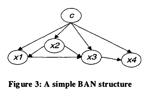
Minimum Description Length (MDL): a scoring function to learn Bayesian Network Structure

Bayesian Network Augmented Naive-Bayes (BAN) is an improved version of Naive-Bayes, in which every attribute $X_i$ may have at most one other attribute as its parent other than the class variable $C$ . For example (figure from [1]):

Though BAN provides a more flexible structure compared to Naive Bayes, the structure (i.e., dependence/independence relationships between attributes) needs to be learnt. [2] proposed a method using a scoring function called Minimum Description Length (MDL) for structure learning. Basically, given training data set $D$ , you start from a random network structure $g_1$ and calculate its $MDL(g_1|D)$ . We set the current best network structure $g^* = g_1$ . Then for any other possible structure $g_i$ , $g_i$ is set to $g^*$ if $MDL(g_i|D) <= MDL(g^*|D)$ . As you can see, we want to find a network structure which can minimize MDL(g|D).

Now let’s look at the exact formula of $MDL(g|D)$ :

$MDL(g|D) = \frac{\log N}{2}|g| - LogLikelihood(g|D)&s=2$

The second term of $MDL(g|D)$ , which is the negative LogLikelihood of $g$ given data $D$ , is easy to understand. Given the data $D$ , we would like the likelihood of such structure $g$ as large as possible. Since we try to minimize $MDL(g|D)$ , we write it in a negative log likelihood format. However, merely using the negative LogLikelihood(g|D) as a scoring function is not enough, since it strongly favors the structure to be too sophisticated (a.k.a, overfitting). That is why the first term $\frac{\log N}{2}|g|$ comes into place to regulate the overall structure:

$|g|$ is the number of parameters in the network. $N$ is the size of dataset. $\frac{\log N}{2}$ is the length of bits to encode every parameter. So $\frac{\log N}{2}|g|$ penalizes the networks with many parameters. Taking for example the network in the figure above, suppose attribute $x_1$ has two possible values, i.e., $x_1 = \{a_1, a_2\}$ . Similarly, $x_2 = \{b_1, b_2, b_3\}$ , $x_3 = \{c_1,c_2\}$ , $x_4 = \{d_1, d_2, d_3, d_4\}$ , and $C=\{o_1, o_2\}$ . Then attribute $x_1, x_2, x_3, x_4$ can have $2\times 3 \times 2 \times 4=48$ combinations of values. Further, we can use one more parameter to represent the joint probability of $P(x_1, x_2, x_3, x_4, C=o_1)$ , one minus which is the joint probability of $P(x_1, x_2, x_3, x_4, C=o_2)$ . Hence $|g| = (|C|-1) \cdot (|x_1| |x_2| |x_3| |x_4|) = 48$ . Why we can use $\frac{\log N}{2}$ bits to encode each parameter? Please refer to section 2 in [3] and my reading note on that at the end of this post.

Back to [2], you can find in the paper that the negative likelihood functino in $MDL$ is replaced by mutual information format. Such transformation is equivalent and was proved in [4].

My reading note on Section 2 in [3]

Until equation (3), the author is just describing the context. Not too hard to understand. Equation (3) basically says there are $k(g)$ number of the parameters in the network. This is exactly what I explained two paragraphs earlier.

Then, the author gave equation (4) (5) (6):

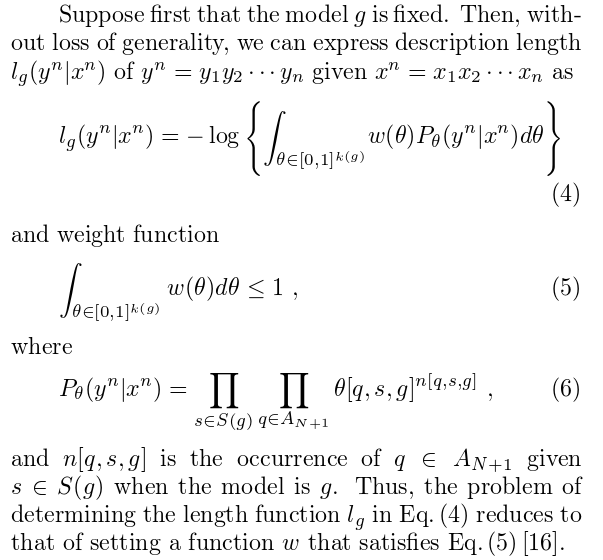
Here, $\theta$ is a vector of length $|k(g)|$ . Each component of vector $\theta$ is noted as $\theta[q,s,g]$ , which refers to the conditional probability of observing $q \in A_{N+1}$ and $s \in S(g)$ given a model $g$ . For a given network $g$ , $\sum_{q}\sum_{s}\theta[q,s,g] =1$ .

Then, $w(\theta)$ is the prior distribution of the vector $\theta$ . The author supposes it is a Dirichlet distribution, thus $w(\theta)$ equals to:

For any possible value $\theta$ , the posterior probability is $w(\theta)P_\theta(y^n|x^n) &s=2$ . The real marginal probaiblity of $P(y^n|x^n)$ is to integrate over all possible $\theta$ values:

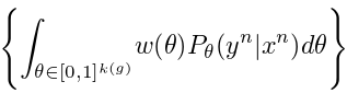
Then the author said the description length of $y^n|x^n$ is just to take negative log as in equation (4). I don’t quite get it at this point. What I can think of is that the negative log likelihood is perfect for its monotonically decreasing property. The higher probability of $P(y^n|x^n)$ , the more desirable the structure is. Since we want to minimize MDL anyway, why not just assign MDL to such negative log format?

Then the author claimed that:

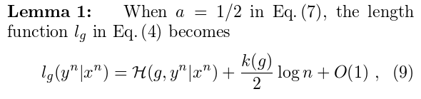
This is why we can use $\frac{\log N}{2}$ bits to encode each parameter.

Reference

[1] Cheng, J., & Greiner, R. (1999, July). Comparing Bayesian network classifiers. In Proceedings of the Fifteenth conference on Uncertainty in artificial intelligence (pp. 101-108). Morgan Kaufmann Publishers Inc..

[2] Hamine, V., & Helman, P. (2005). Learning optimal augmented Bayes networks. arXiv preprint cs/0509055.

[3] Suzuki, J. (1999). Learning Bayesian belief networks based on the minimum description length principle: basic properties. IEICE transactions on fundamentals of electronics, communications and computer sciences, 82(10), 2237-2245.

[4] Friedman, N., Geiger, D., & Goldszmidt, M. (1997). Bayesian network classifiers. Machine learning, 29(2-3), 131-163.

Other references, though not used in the post, are useful in my opinion:

[5] De Campos, L. M. (2006). A scoring function for learning bayesian networks based on mutual information and conditional independence tests. The Journal of Machine Learning Research, 7, 2149-2187.

[6] Rissanen, J. (1978). Modeling by shortest data description. Automatica, 14(5), 465-471.

[7] Liu, Z., Malone, B., & Yuan, C. (2012). Empirical evaluation of scoring functions for Bayesian network model selection. BMC bioinformatics, 13(Suppl 15), S14.

Minimum Description Length (MDL): a scoring function to learn Bayesian Network Structure

Leave a comment

Cancel reply