Learn GPU Optimization

It has been a while since I learned GPU knowledge. I am going to keep updating more recent materials for ramping up my GPU knowledge.

FlashAttention [1]

We start from recapping the standard Self-Attention mechanism, which is computed in 3-passes:

Notes:

1. The shape and represent the sequence length and internal dimension, respectively. , , , which transform token embeddings into a projected latent space.
2. is the attention matrix. represents how much attention token should pay for . In normal LLM tasks, we will apply a causal mask so that only is valid, because a token can only pay attention to all previous tokens. The softmax() operator is applied per-row of .
3. The output represents the weighted values from other tokens per position. will be fed to feed forward layers to be transformed into output space (from shape to ). We omit the part after self-attention.

How GPUs work is that GPUs have a massive number of threads to execute an operation (called a kernel). Each kernel loads inputs from HBM to registers and SRAM, computes, then writes outputs to HBM. HBM has larger storage but slower speed. In practice, the times of HBM accesses play a non-negligible role in GPU execution speed. 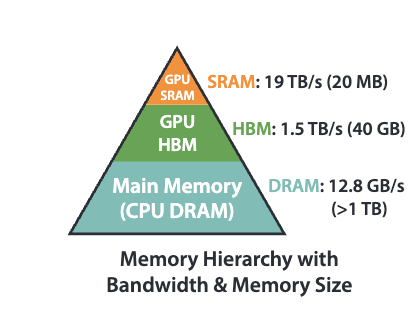In standard self-attention, it requires HBM accesses, because we need to load , , and from HBM and we need to read/write of and , each of shape . 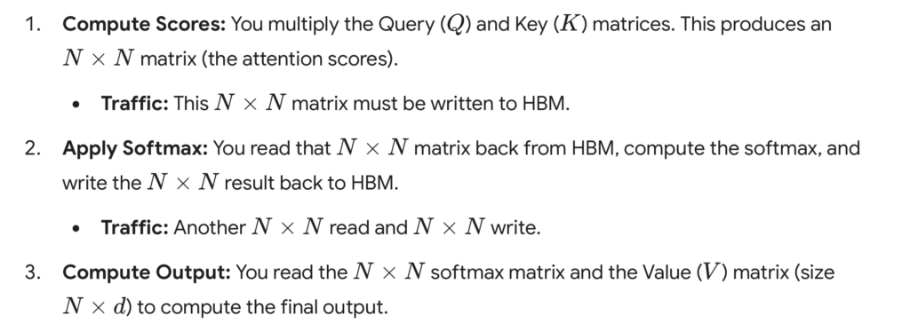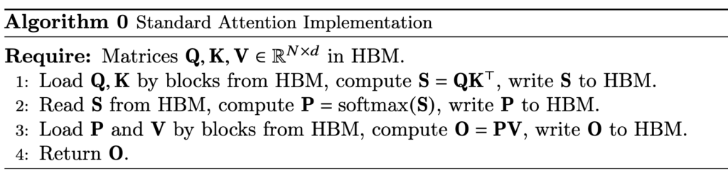A detailed breakdown of standard self-attention HBM accesses is as below (illustrated by Gemini): Let’s dive into the step of computing softmax. Even computing softmax has many details. First, in real world, we usually need to compute a safe softmax version, where we subtract each input to the softmax with the maximum input to avoid potential overflow. (Diagrams from [3]) 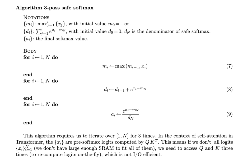In its vanilla implementation, we need to have three passes: the first pass computes the maximum of the input, the second pass computes the denominator of the softmax, and the third pass computes the actual softmax. Asymptotically these three steps require time but in reality the constant factor of the computation is also important. SRAM is typically too small to hold the -size result. So we either need to save into HBM in the first pass and load it in the following two steps, or even need to recompute , depending whichever is faster. That means this three-passes safe softmax algorithm does require computation time / accesses to HBM. It turns out that we can turn the 3-passes algorithm into 2-passes. This is something called online softmax. As we traverse each , we can record the maximum value so far and the accumulative softmax denominator. The accumulative softmax denominator from the previous can be easily scaled whenever a new maximum is found at . 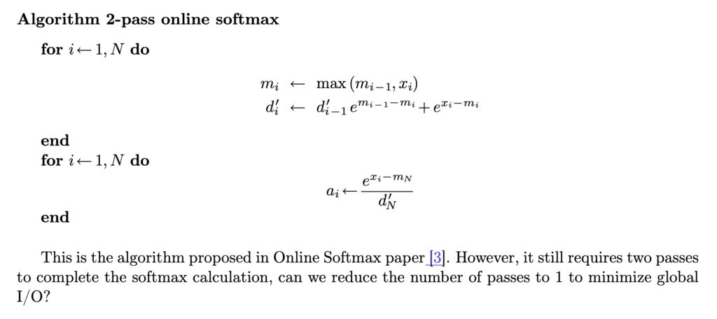With this 2-pass online softmax algorithm, self-attention can also be computed in two-passes: 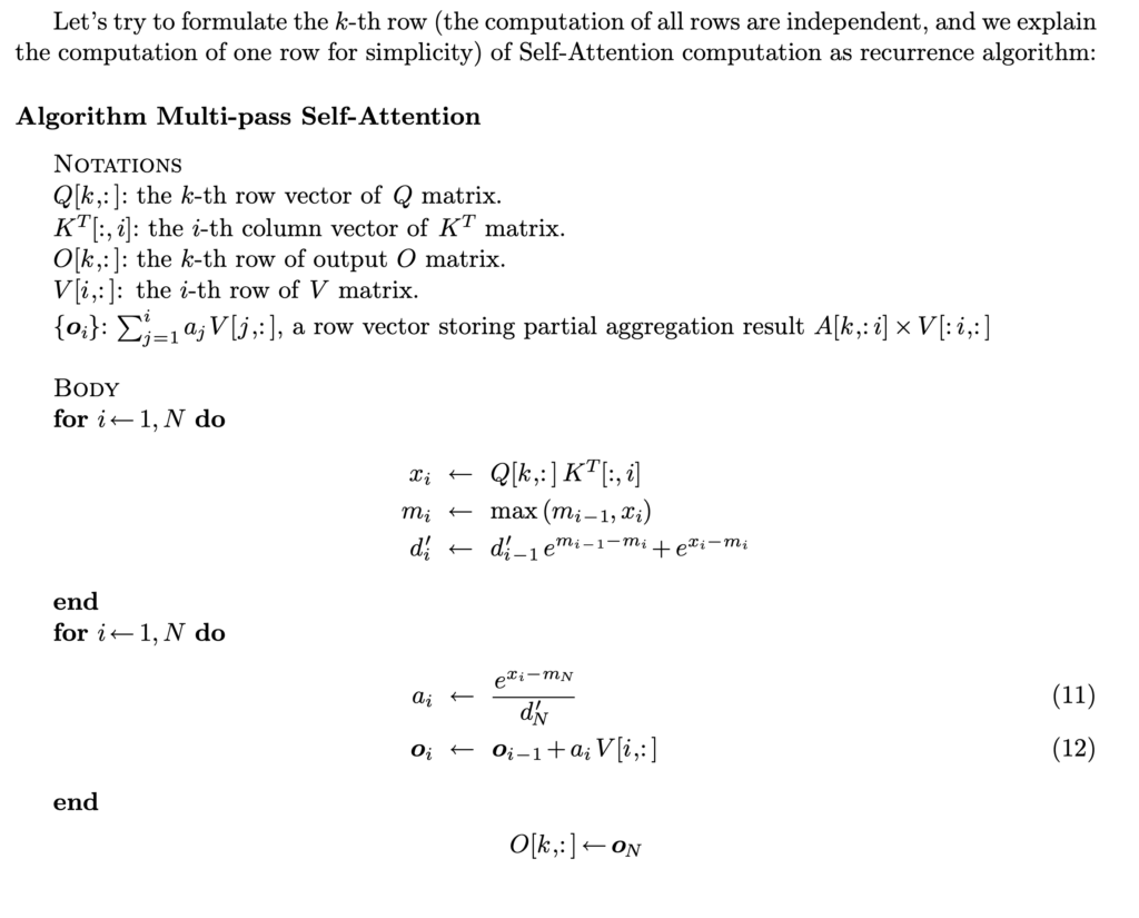However, we can do better by finding that can also be computed “online” together with the running maximum value and running accumulative softmax denominator . 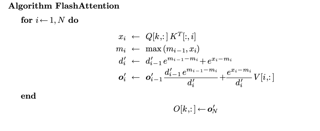That’s how we end up with FlashAttention which requires one pass to compute the output vectors! 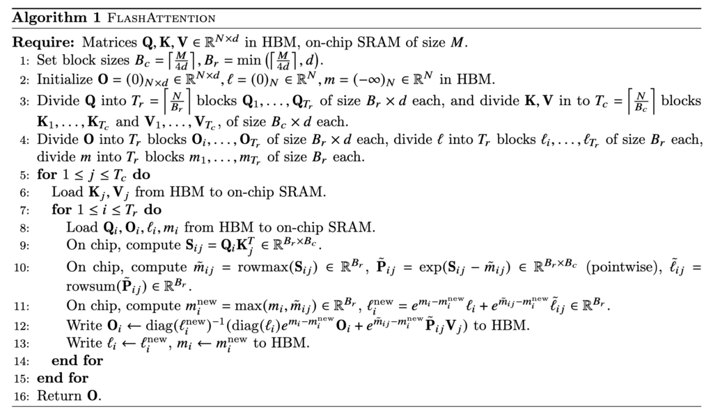In reality, a further optimization is to load Q/K/V in blocks so that the blocks of Q, K, V, and O can occupy roughly the full SRAM memory at one time. That’s why we see block size is set at or in the algorithm. 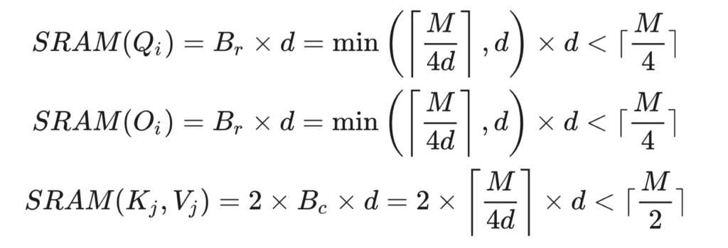Now, we examine how to do backward computation in FlashAttention. We start from examining the standard attention backward pass: 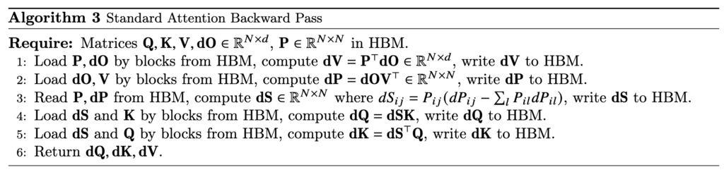(To clarify the notations, is the gradient of the loss with respect to the attention output matrix, i.e., , which has the same shape as . Similarly for , , and . We also assume is already available as the backpropagation computation has been done from to ) Let’s try to understand this standard backward pass:

1. With , due to matrix calculus rules, we have .
2. We need to compute and record because it will be used in computing and . Due to matrix calculus rules, we have .
3. . There is a well-known mathematical result stating that the Jacobian matrix of softmax can be computed by , where is a row of . With some simplification, we reach to . [Note: while is a row of (and is a row of ), it is still treated a column vector following the convention of linear algebra. So is actually a scalar, an inner product, while is a matrix, an outer product, of the two vectors.]
4. With and matrix calculus rules, we obtain and .

As we can see, the standard attention backward pass requires loading , , , , , , and writing , , , , and . However, in FlashAttention we do not store . So in its backward pass, we also need to compute (blocks of) on the fly. Moreover, can be computed and prestored in HBM via and :

(1)  

1. Forward pass:
   1. standard attention: as discussed above
   2. FlashAttention: because one full inner loop (starting from line 7 in Algorithm 1) needs to load the full from HBM (), and the outer loop (line 5 in Algorithm 1) needs to perform times (). Another good reference of IO complexity analysis can be found in [4]
2. Backward pass:
   1. standard attention:
   2. FlashAttention: Please see analysis in Theorem 5 in [1]

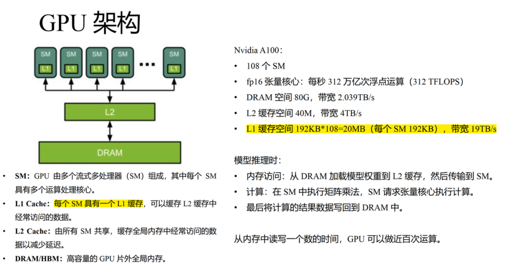
In practice, when will FlashAttention outperform Attention? This is when can be greatly smaller than . First of all, we need to clarify that should represent the L1 cache size of one streaming multiprocessor (SM) in a GPU. Taking A100 as an example, one SM has 192KB L1 cache. So FlashAttention will probably have advantage of IO complexity when 64, 128, or 256 but has no advantage when . Let’s also summarize the total memory footprint required by standard attention vs FlashAttention: 1. standard attention: it needs to store , , and matrices, which needs space. However the most costly part comes from storing and , which takes space. Overall, the memory footprint is . 2. FlashAttention: it still needs to store , , and matrices, which needs space. But it does not store and ; instead it maintains the running maximum values and running accumulative softmax denominators in the forward pass so that they can be used in the backward pass, which takes space. Overall, the memory footprint of FlashAttention is only .    

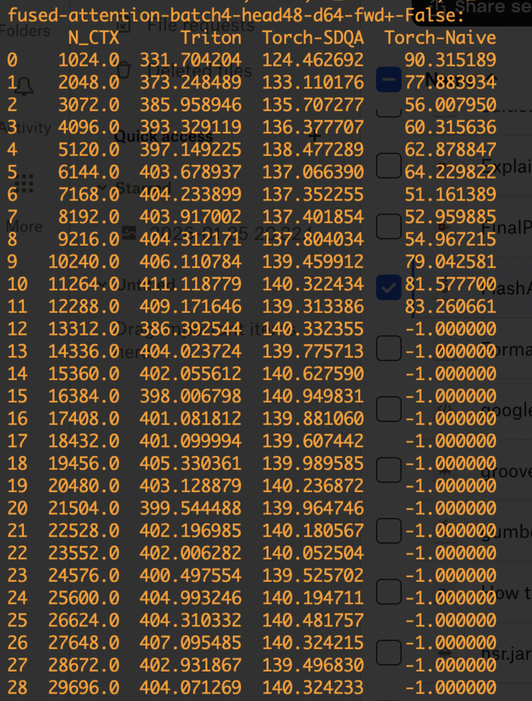
Now let’s move on to the engineering test. I picked one simple online implementation of FlashAttention and compared it with pytorch scaled dot product attention implementation (with backend=memory efficient) and a naive implementation of attention. Note that FlashAttention can be thought as a combination of reducing memory as HBM accesses. The pytorch implementation with the memory efficient backend essentially only reduces the memory footprint but not HBM accesses. The comparing script is here (python benchmark_flash_triton.py).

The comparison result is shown below. The numbers are TFlops measured. We test both forward and backward passes under the setting: num_heads = 48 and num_dim = 64. When OOM arises, we mark the result as -1. We can see the FlashAttention version clearly has higher FLOPs and can handle much longer sequences than the other two versions.

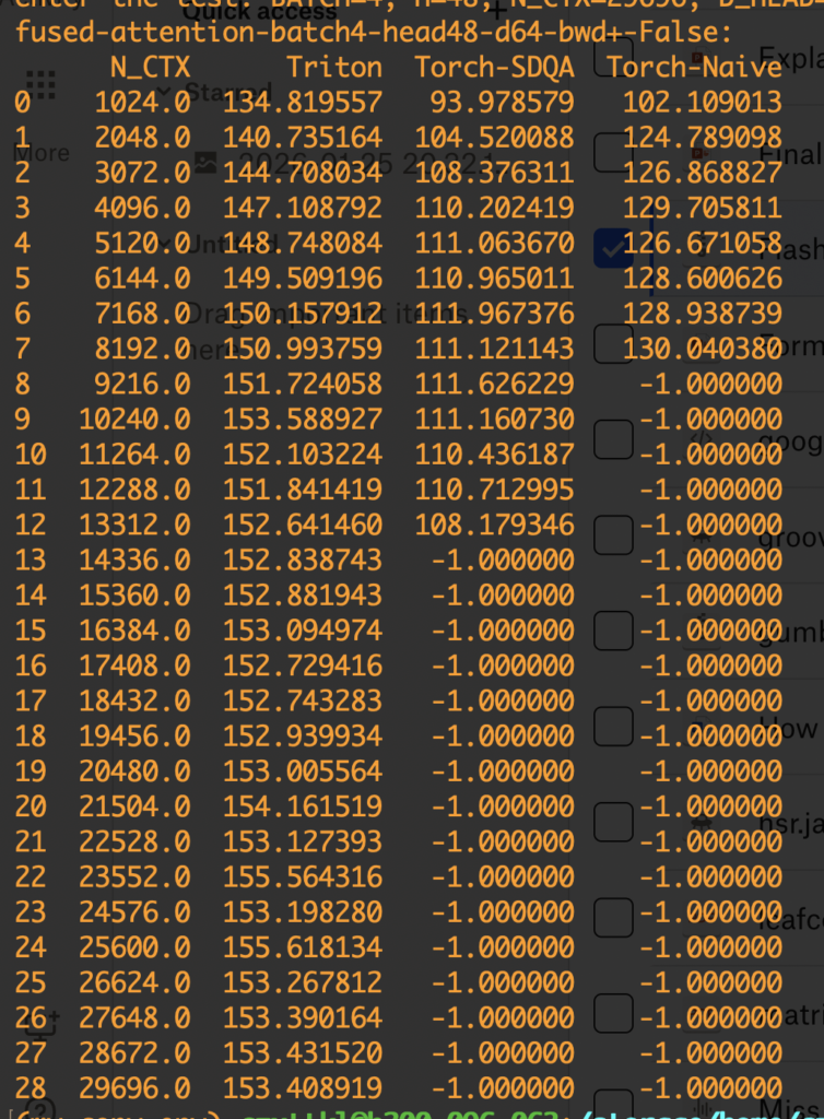
As a technique to reduce memory footprint and HBM accesses, FlashAttention is useful in training and the pre-filling stage in inference, both requiring obtaining the attention outputs of given sequences. So FlashAttention can be helpful to reduce time-to-first-token (TTFT). However, for the actual decoding phase, we need more pecialized variants (like Flash-Decoding). We will cover it later.

Torch.compile / CudaGraph

Cuda Graphs is an NVIDIA hardware-level optimization designed to speed up communication delay between CPU and GPU because sometimes your computation speed may be bottlenecked by how fast CPU sends kernel launch commands to GPU. The Cuda Graphs technique captures the kernel launch sequences in a graph structure first and then in the replay phase the CPU can just send one single command to GPU to execute the graph, which consists of all recorded kernel launches. Torch.compile is a set of optimization techniques that can be automatically applied to python+pytorch functions. It records python code logics in computation graphs and then rely on TorchInductor to conduct optimizations:

1. fuse operations/kernels
2. auto-tune kernel configurations like block sizes
3. Choose different backends for matmul and perform prologue and epilogue fusion (TODO: understand these fusions)
4. use CUDA Graphs to cache and replay kernel launches efficiently

As you can see, torch.compile is a superset of optimization techniques like Cuda Graphs. Below, we show a very basic example of how torch.compile accelerates a function. We test two modes of torch.compile, “max-autotune” and “max-autotune-no-cudagraphs”. While max-autotune gives torch.compile the full autonomy to compile your function, sometimes it may over-engineer it. For example, applying cuda graphs may be overkill for small functions like the one in the example below.

import torch
import time
import torch._dynamo as dynamo

# Ensure you have a CUDA-enabled GPU for the best results
device = 'cuda' if torch.cuda.is_available() else 'cpu'
print(f"Using device: {device}")

# 1. Define a simple function with a loop
def my_function(x):
    for _ in range(10):
        # A series of simple operations
        x = torch.sin(x) + torch.cos(x)
    return x

# 2. Create some input data
input_tensor = torch.randn(1024, 1024, device=device)

# 3. Compile the function
# The 'mode' can be tuned for different trade-offs. 'max-autotune' is aggressive.
compiled_function = torch.compile(my_function, mode="max-autotune")

# 4. Compile the function without cuda graph
# The 'mode' can be tuned for different trade-offs. 'max-autotune' is aggressive.
compiled_function_no_cuda_graph = torch.compile(my_function, mode="max-autotune-no-cudagraphs")

# --- Benchmarking ---

# WARM-UP RUNS: The first run has a one-time compilation overhead.
# We run both once to get this out of the way for fair timing.
print("\nStarting warm-up runs...")
_ = my_function(input_tensor)
_ = compiled_function(input_tensor)
_ = compiled_function_no_cuda_graph(input_tensor)
if device == 'cuda':
    torch.cuda.synchronize()
print("Warm-up complete.")


# Time the original EAGER mode function
print("\nBenchmarking Eager Mode...")
start_time = time.perf_counter()
for _ in range(100):
    _ = my_function(input_tensor)
# Make sure all GPU operations are finished before stopping the timer
if device == 'cuda':
    torch.cuda.synchronize()
eager_time = time.perf_counter() - start_time


# Time the COMPILED function
print("Benchmarking Compiled Mode...")
start_time = time.perf_counter()
for _ in range(100):
    _ = compiled_function(input_tensor)
if device == 'cuda':
    torch.cuda.synchronize()
compiled_time = time.perf_counter() - start_time


# Time the COMPILED function with no cuda graph
print("Benchmarking Compiled Mode with no Cuda Graphs...")
start_time = time.perf_counter()
for _ in range(100):
    _ = compiled_function_no_cuda_graph(input_tensor)
if device == 'cuda':
    torch.cuda.synchronize()
compiled_time_no_cuda_graph = time.perf_counter() - start_time


# --- Results ---
print("\n--- Results ---")
print(f"Eager mode total time:    {eager_time:.4f} seconds")
print(f"Compiled mode total time: {compiled_time:.4f} seconds")
print(f"Compiled mode with no cuda graph total time: {compiled_time_no_cuda_graph:.4f} seconds")
print(f"\nSpeedup: {eager_time / compiled_time:.2f}x faster! 🎉")
print(f"Speedup with no cuda graph: {eager_time / compiled_time_no_cuda_graph:.2f}x faster! 🎉")


# Use explain to see how Dynamo will handle the function
# It will print out a detailed report
explanation = dynamo.explain(my_function)(input_tensor)
print("\n" + "="*50)
print("Dynamo Explanation Output Summary:")
print(explanation)

Eager mode total time:    0.0157 seconds
Compiled mode total time: 0.0856 seconds
Compiled mode with no cuda graph total time: 0.0025 seconds

Speedup: 0.18x faster! 
Speedup with no cuda graph: 6.32x faster!