In this post I am showing my understanding about the paper Adaptive Regularization of Weight Vectors: http://papers.nips.cc/paper/3848-adaptive-regularization-of-weight-vectors.pdf
The paper aims to address the negatives of a previous algorithm called confidence weighted (CW) learning by introducing the algorithm Adaptive Regularization Of Weights (AGOW). CW and AGOW are both online learning algorithms, meaning updates happen after observing each datum. The background under investigation is linear binary classifier, i.e., the algorithms try to learn weights $latex \boldsymbol{w}$ such that ideally given a datum $latex \boldsymbol{x}_t$ and its real label $latex y_t$, $latex sign(\boldsymbol{w} \cdot \boldsymbol{x}_t) = y_t$.
First, let’s look at the characteristics of CW. At each round $latex t$ where a new datum $latex (\boldsymbol{x}, y_t)$ is observed, CW aims to solve the following optimization problem:
$latex (\boldsymbol{\mu}_t, \Sigma_t) = \min\limits_{\boldsymbol{\mu}, \Sigma} D_{KL}(\mathcal{N}(\boldsymbol{\mu}, \Sigma) || \mathcal{N}(\boldsymbol{\mu}_{t-1}, \Sigma_{t-1})) \\ \qquad \qquad \text{ s.t. } Pr_{\boldsymbol{w} \sim \mathcal{N}(\boldsymbol{\mu}, \Sigma)}[y_t (\boldsymbol{w} \cdot \boldsymbol{x}_t) \geq 0] \geq \eta $
Interpreted in plain English, the optimization problem of CW says: I should make sure the current example can be predicted correctly with $latex \eta$ confidence by updating the underlying distribution of weights $latex \boldsymbol{w}$. However, the update should be as little as possible to preserve previous weights as much as possible.
The paper analyzes the positives and the negatives of CW: forcing the probability of predicting each example correctly to be at least $latex \eta$ (usually $latex > \frac{1}{2}$) can lead to rapid learning but suffer over-fitting problem if labels are very noisy. Also, the constraint, $latex Pr_{\boldsymbol{w} \sim \mathcal{N}(\boldsymbol{\mu},\Sigma)}[y_t (\boldsymbol{w} \cdot \boldsymbol{x}_t) \geq 0] \geq \eta$, is specific to linear binary classification problems, leaving people unknown how to extend to alternative settings.
The paper proposes AGOW with the following unconstrained optimization problem:
$latex C(\boldsymbol{\mu}, \Sigma) = D_{KL}(\mathcal{N}(\mu, \Sigma) || \mathcal{N}(\mu_{t-1}, \Sigma_{t-1}) ) + \lambda_1 \ell_{h^2}(y_t, \boldsymbol{\mu} \cdot \boldsymbol{x}_t) + \lambda_2 \boldsymbol{x}_t^T \Sigma \boldsymbol{x}_t \\ \text{ where } \ell_{h^2}(y_t, \boldsymbol{\mu} \cdot \boldsymbol{x}_t) = (\max \{ 0, 1 – y_t (\boldsymbol{\mu} \cdot \boldsymbol{x}_t) \} )^2 \text{ is a squared hinge loss function. }$
The optimization problem of AGOW aims to balance the following desires:
- each update should not be too radical. (the first KL divergence term)
- the current datum should be predicted with low loss. (the second term). The property of the hinge loss indicates that if the current datum can be predicted correctly with sufficient margin (i.e., $latex y_t(\boldsymbol{\mu}\cdot \boldsymbol{x}_t) > 1$) before updating the parameters, then there is no need to update $latex \boldsymbol{\mu}$.
- confidence in the parameters should generally grow. (the third term). Note that covariance matrix is always positive semi-definite as you can google it.
Now I will show how to derive the update rule for $latex \boldsymbol{\mu}$. Since $latex C(\boldsymbol{\mu}, \Sigma)$ is a convex function w.r.t. $latex \boldsymbol{\mu}$ and it is differentiable when $latex 1 – y_t(\boldsymbol{\mu}_t \cdot \boldsymbol{x}_t) \geq 0$, we can update $latex \boldsymbol{\mu}$ by setting the derivative of $latex C(\boldsymbol{\mu}, \Sigma)$ w.r.t to $latex \boldsymbol{\mu}$ to zero:
$latex \frac{\partial C(\boldsymbol{\mu}, \Sigma)}{\partial\boldsymbol{\mu}} = \frac{\partial}{\partial\boldsymbol{\mu}} \frac{1}{2}(\boldsymbol{\mu}_{t-1} -\boldsymbol{\mu})^T \Sigma_{t-1}^{-1}(\boldsymbol{\mu}_{t-1} -\boldsymbol{\mu}) + \frac{\partial}{\partial \boldsymbol{\mu}} \frac{1}{2r} \ell_{h^2}(y_t, \boldsymbol{\mu} \cdot \boldsymbol{x}_t) = 0$
Rearranging the equality above we can get formula (6) in the paper:
$latex \boldsymbol{\mu}_t = \boldsymbol{\mu}_{t-1} + \frac{y_t}{r}(1-y_t (\boldsymbol{x}_t^T \boldsymbol{\mu}_t)) \Sigma_{t-1} \boldsymbol{x}_t$
If we multiply both sides by $latex \boldsymbol{x}_t^T$, we get:
$latex \boldsymbol{x}_t^T \boldsymbol{\mu}_t = \boldsymbol{x}_t^T \boldsymbol{\mu}_{t-1} + \frac{y_t}{r}(1-y_t (\boldsymbol{x}_t^T \boldsymbol{\mu}_t)) \boldsymbol{x}_t^T \Sigma_{t-1} \boldsymbol{x}_t$
Moving everything containing $latex \boldsymbol{x}_t^T \boldsymbol{\mu}_t$ to the left we get:
$latex (1+ \frac{1}{r}\boldsymbol{x}_t^T \Sigma_{t-1} \boldsymbol{x}_t) \boldsymbol{x}_t^T \boldsymbol{\mu}_t = \frac{y_t}{r}\boldsymbol{x}_t^T \Sigma_{t-1} \boldsymbol{x}_t + \boldsymbol{x}_t^T \boldsymbol{\mu}_{t-1}$
Therefore,
$latex \boldsymbol{x}_t^T \boldsymbol{\mu}_t = \frac{y_t \boldsymbol{x}_t^T \Sigma_{t-1} \boldsymbol{x}_t + r \boldsymbol{x}_t^T \boldsymbol{\mu}_{t-1}}{r+\boldsymbol{x}_t^T \Sigma_{t-1} \boldsymbol{x}_t}$
Plugging the formula above back to where $latex \boldsymbol{x}_t^T \boldsymbol{\mu}_t$ appears in formula (6), we have:
$latex \boldsymbol{\mu}_t = \boldsymbol{\mu}_{t-1} + \frac{1 – y_t \boldsymbol{x}_t^T \boldsymbol{\mu}_{t-1}}{r+\boldsymbol{x}_t^T \Sigma_{t-1} \boldsymbol{x}_t} \Sigma_{t-1} y_t \boldsymbol{x}_t$
Recall the passive way AGOW adopts to update $latex \boldsymbol{\mu}_t$:
- if $latex 1 – y_t(\boldsymbol{\mu}_t ) < 0$, which means the margin to predict this datum is already large enough, there is no need to update $latex \boldsymbol{\mu}_t$, i.e. $latex \boldsymbol{\mu}_t = \boldsymbol{\mu}_{t-1}$.
- if $latex 1 – y_t(\boldsymbol{\mu}_t ) \geq 0$ then we need to update $latex \boldsymbol{\mu}$ according to the equality above.
To combine these two update rules, we obtain the formula (7) in the paper:
$latex \boldsymbol{\mu}_t = \boldsymbol{\mu}_{t-1} + \frac{\max(0, 1 – y_t \boldsymbol{x}_t^T \boldsymbol{\mu}_{t-1})}{r+\boldsymbol{x}_t^T \Sigma_{t-1} \boldsymbol{x}_t} \Sigma_{t-1} y_t \boldsymbol{x}_t$
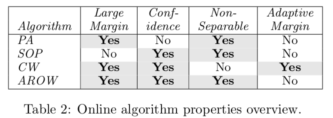
I skip the derivation for the update rule of $latex \Sigma$. The most important conclusion of the paper can be found in Table 2 where it summarizes pros and cons of state-of-the-art online learning algorithm.
