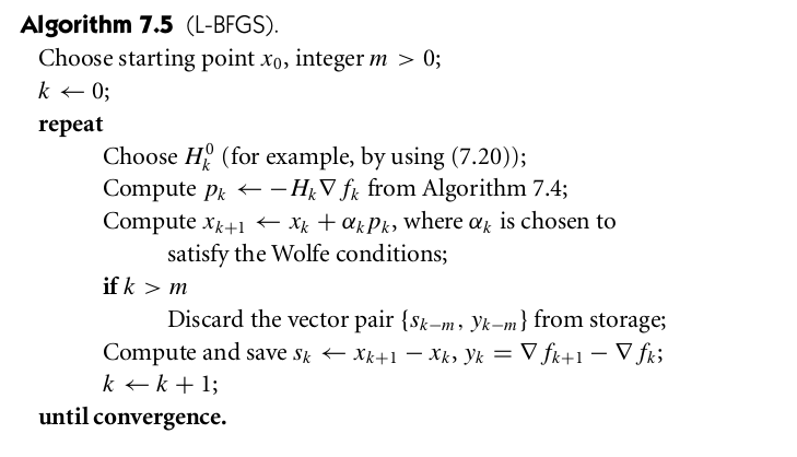
Good explanation for BFGS and L-BFGS can be found in this textbook: https://www.dropbox.com/s/qavnl2hr170njbd/NumericalOptimization2ndedJNocedalSWright%282006%29.pdf?dl=0
In my own words:
Gradient descent and its various variants have been proved to learn parameters well in practical unconstrained optimization problems. However, it may converge too slowly or too roughly depending on how you set learning rate.
Remember the optimum in unconstrained optimization has zero first derivative. Newton (and Raphson) method uses tangent information of first derivative (i.e., second derivative) to find root of first derivative (i.e., the value making first derivative equal to zero). It usually converges in a quadratic convergence rate (if classic assumptions of Newton method are satisfied). However, in every iteration of Newton method for a multivariate unconstrained optimization, not only the Hessian matrix but its inversion need to be calculated, which prohibits from Newton method being applied to high dimension problems.
BFGS, as a member of quasi-Newton method family, uses cheaper calculation to approximate inversion of Hessian. But it is still expensive in respect of memory usage. Later, L-BFGS was coined to use thrift memory to achieve comparable precision as BFGS does.
My notes in implementing L-BFGS:
We use the same notation as in the textbook written by Jorge Nocedal:
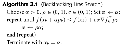
You need to use line search to determine $latex \alpha_k$. Simple backtracking line search is not going to work because $latex p_k$ should satisfy both Wolfie conditions.
People have designed different versions of line search to meet both Wolfie conditions (see: https://www.math.lsu.edu/~hozhang/papers/nonmonotone.pdf and https://github.com/JuliaOpt/Optim.jl/issues/26), I am using a simple version:
- if 3.6a is not satisfied, reduce $latex \alpha_k$ by half in every line search iteration.
- when 3.6a is satisfied, double $latex \alpha_k$ until 3.6b is satisfied.
When you determine $latex p_k$, you can also check if $latex \nabla(f_k) p_k = \nabla(f_k) H_k \nabla(f_k)> 0$. $latex H_k$ in every iteration in BFGS should be positive definite because:
H should be positive definite, so that f(x) reaches local minimum at $latex H^{-1} p$.
https://en.wikipedia.org/wiki/Hessian_matrix#Second_derivative_test
Reference
http://www.alglib.net/optimization/lbfgsandcg.php
http://aria42.com/blog/2014/12/understanding-lbfgs/
http://andrew.gibiansky.com/blog/machine-learning/hessian-free-optimization/
http://papers.nips.cc/paper/5333-large-scale-l-bfgs-using-mapreduce.pdf


